LASSO Regression:
Mastering Feature Selection for Predictive Models

---

LASSO - short introduction

LASSO (Least Absolute Shrinkage and Selection Operator), similar to ridge regression, is a certain modification of linear regression. As we remember from the article "From Theory to Practice: Ridge Regression for Improved Predictive Models", ridge regression is specifically designed to address multicollinearity in the dataset. The LASSO method has a completely different but also useful advantage. It performs both feature selection and regularization in order to enhance the prediction accuracy and interpretability of the resulting model.

Feature selection in machine learning involves selecting a subset of relevant features (or variables) from the original set of features available in the dataset. The goal of feature selection is to improve model performance by reducing the dimensionality of the feature space, removing irrelevant or redundant features, and focusing only on those features that contribute most to the predictive power of the model.

Regularization refers to the technique of adding a penalty term to the objective function during training to prevent overfitting and improve generalization performance.
The primary goal of regularization is to discourage the model from fitting the training data too closely, which can lead to poor performance on unseen data.

Ridge regression also introduces a regularization term that penalizes large coefficients. In the case of ridge regression, the regularization term is known as the L2 penalty. In LASSO, the regularization term has a slightly different form and is called the L1 penalty.

Put simply, both penalty terms serve a similar regularization purpose, but their differing mathematical forms cause them to influence the model in distinct ways. Moreover, each penalty has its own characteristic properties.

Linear Regression - one more time!

In short, in linear regression, the goal is to minimize a certain expression (RSS) with respect to the parameter values \(\beta_i\). $$\arg \min_{\beta_0,..., \beta_p} \quad \sum_{i=1}^{n}\left( y_i-\beta_0-\sum_{j=1}^{p}\beta_jx_{ij} \right)^2$$ Let's see how for the LASSO model, the expression we minimize is different.

LASSO - definition

In LASSO, we also minimize the RSS, however, augmented by a regularization term called the L1 penalty. $$\arg \min_{\beta_0,..., \beta_p} \quad \sum_{i=1}^{n}\left( y_i-\beta_0-\sum_{j=1}^{p}\beta_jx_{ij} \right)^2+\lambda\sum_{j=1}^{p}|\beta_{j}|$$ Astute readers will surely recognize the parameter \(\lambda\) and associate it with other methods we have already described on our blog. The parameter \(\lambda\) is a tuning parameter that determines how much penalty we impose on the model for having excessively large coefficients.

In LASSO regression, the regularization parameter \(\lambda\) controls how strongly the model is penalized for using many or large coefficients. If \(\lambda\) is set too small, the penalty becomes almost negligible and the model behaves similarly to ordinary linear regression, which increases the risk of overfitting. Conversely, if \(\lambda\) is chosen too large, many coefficients are shrunk aggressively towards zero, leading to an excessively simple model that may fail to capture relevant patterns in the data, resulting in underfitting.
To balance this trade-off, \(\lambda\) is typically selected using cross-validation. A very similar discussion of this bias-variance trade-off and the role of cross-validation in choosing the regularization strength was presented in the article "From Theory to Practice: Ridge Regression for Improved Predictive Models". Readers interested in a more detailed explanation of how cross-validation curves are constructed, how to interpret them, and how different \(\lambda\) values affect model complexity are encouraged to refer to that article for additional background and intuition.

What is the difference between LASSO and Ridge Regression?

Let's remind the form of the expression we minimize in the case of ridge regression model: $$\arg \min_{\beta_0,..., \beta_p} \quad \sum_{i=1}^{n}\left( y_i-\beta_0-\sum_{j=1}^{p}\beta_jx_{ij} \right)^2+\lambda\sum_{j=1}^{p}\beta_{j}^2$$ Notice that the difference between ridge regression and LASSO models appears to be very small. It only lies in the fact that the regularization term has a slightly different form. In fact, the expression we minimize in these models only differs in the norm we use for the penalty. In ridge regression, we used the norm \(p=2\), while in LASSO we use the norm \(p=1\).

Norm
Let \( X \) be a vector space over the field \( K \). Function \( \|\cdot\|: X \longrightarrow \mathbb{R}_{+} \) is called a norm on \( X \) if:
(1) For all \( x \) in \( X \), \( \|x\| = 0 \) if and only if \( x = 0 \) (positive definiteness).
(2) For all \( x \) in \( X \) and \( \alpha \) in \( K \), \( \|\alpha x\| = |\alpha| \cdot \|x\| \) (absolute homogeneity).
(3) For all \( x, y \) in \( X \), \( \|x+y\| \leq \|x\| + \|y\| \) (triangle inequality).

\(p\)-norm is defined as:
$$||x||_p=(|x_1|^{p}+|x_2|^{p}+...+|x_n|^{p})^{1/p}$$ Example of \(p\)-norm for \(p=1\) and \(p=2\): $$||x||_1=|x_1|+|x_2|+...+|x_n|$$ $$||x||_2=\sqrt{x_1^{2}+x_2^2+...+x_n^2}$$

Below we present charts of balls in different norms:

Why LASSO shrink coefficients exactly to zero?

In many textbooks and articles, the difference between LASSO and ridge regression is illustrated using the shapes of the L1 and L2 norms. Ridge regression uses the L2 norm, whose constraint region in two dimensions is a circle, while LASSO uses the L1 norm, whose constraint region is a diamond (a rotated square). The residual sum of squares (RSS) is represented by elliptical contour lines centered around the ordinary least squares solution, and the regularized solution is found at the point where the smallest RSS contour touches the constraint region.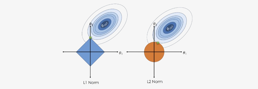


The key geometric insight is that the L1 diamond has sharp corners lying exactly on the coordinate axes, whereas the L2 circle is smooth everywhere. As the RSS ellipses expand outward until they first intersect the L1 constraint region, they very often touch the diamond exactly at one of these corners. Each corner corresponds to a point where at least one coefficient is exactly zero. In higher dimensions, the L1 ball becomes a polytope with many such corners (edges and vertices), and the optimal solution tends to lie on these lower-dimensional faces, which again means that many coefficients are driven precisely to zero.

In contrast, the smooth, round shape of the L2 constraint makes it much less likely that the first point of contact with an RSS contour will fall exactly on an axis. As a result, ridge regression usually shrinks coefficients towards zero but almost never makes them exactly zero, while LASSO naturally produces sparse solutions with true zeros.


Now we know what the objective function for the LASSO method looks like. In the next section, we will try to figure out how to optimize this function to find the best model parameters.

Bad news - no closed solution for LASSO

One might want to say that the task is simple and that we can use optimization tools exactly like in the case of previous linear regression and ridge regression models. Unfortunately, that is absolutely not the case.
To worry you even more, I'd say that in general, there is no closed-form solution. 😔

In previous cases, we looked for a minimum point where the derivative of objective function equals zero. However, now, due to the form of the regularization term (\(\lambda\sum_{j=1}^{p}|\beta_{j}|\)), our objective function is no longer differentiable!

Since we can't find a closed-form solution, we need to change our approach. It might be a good idea to use one of the iterative methods. However, it's worth noting that most of them, such as gradient descent or Newton's method, also require the function to be differentiable, which unfortunately ours is not.
So, how do we deal with our optimization problem?

Since ordinary differentiation doesn't work, maybe we should try subdifferentiation? Additionally, the multidimensionality of our function doesn't help us at all. Perhaps if we can focus on just one dimension at a time, the matter will be simpler?

Yes, and the key to an effective solution for LASSO became the coordinate descent algorithm.

Fun Fact!
In 1997, Tibshirani's student Wenjiang Fu at the University of Toronto develops the shooting algorithm for the lasso, but Tibshirani doesn't fully appreciate it.
Some years later, in 2002, Ingrid Daubechies gives a talk at Stanford, describing a one-at-a-time algorithm for the lasso. Trevor Hastie implements it, makes an error, and together with Tibshirani, they conclude that the method doesn't work.
In 2006, Friedman is the external examiner at the PhD oral exam of Anita van der Kooij, who uses coordinate descent for elastic net. Professors are forced to revisit the problem.
Perhaps the shooting algorithm wasn't such a bad idea after all?

What is coordinate descent?

Here's a quick high-level overview of the coordinate descent algorithm:

(1) Start with an initial guess for the parameters \(\mathbf{x} = (x_1^0,...,x_p^0)\)
(2) For each parameter \(k=1,...,p\):
\(\hspace 8mm\) (2.1) Iteratevly solve the single variable optimization problem:
$$\mathbf{x}_i = \arg \min_{\omega} f(x_1, ..., x_{i-1}, \omega, x_{i+1}, ..., x_p)$$ \(\hspace 8mm\) (2.2) Update the parameter in a way that minimizes the objective function with respect to that parameter alone and repeat this process for each parameter until convergence criteria are met.

The key idea behind coordinate descent is that, for many optimization problems, updating one parameter at a time can be simpler and more computationally efficient than updating all parameters simultaneously. This approach is particularly well-suited for problems with a large number of parameters or when the objective function is not differentiable or not easily optimized using gradient-based methods.

Coordinate descent + Subderivative = Success

Let's split our objective function into two parts: $$RSS = \sum_{i=1}^{n}\left( y_i-\beta_0-\sum_{j=1}^{p}\beta_jx_{ij} \right)^2$$ $$L_1 = \lambda\sum_{j=1}^{p}|\beta_{j}|$$ The first part, RSS, is differentiable, and we know how to optimize it using differential calculus.
The problematic part is the \(L_1\). However, it's not that bad. Our function is not differentiable only at one point - \(\beta=0\).

The combination of coordinate descent and subderivative will allow us to deal with optimizing the objective function for LASSO.

Subderivative
Rigorously, a subderivative of a convex function \(f:I\to \mathbb {R}\) at a point \(x_{0}\) in the open interval \(I\) is a real number \(c\) such that for all \(x\in I\) $$f(x)-f(x_{0})\geq c(x-x_{0})$$ By the converse of the mean value theorem, the set of subderivatives at \(x_{0}\) for a convex function is a nonempty closed interval \([a,b]\) where \(a\) and \(b\) are the one-sided limits $$a=\lim _{x\to x_{0}^{-}}{\frac {f(x)-f(x_{0})}{x-x_{0}}}$$ $$b=\lim _{x\to x_{0}^{+}}{\frac {f(x)-f(x_{0})}{x-x_{0}}}$$ The interval \([a,b]\) of all subderivatives is called the subdifferential of the function \(f\) at \(x_{0}\) denoted by \(\partial f(x_{0})\).

How to estimate coefficients in LASSO?

Since in each step of the coordinate descent algorithm we optimize the objective function with respect to only one coordinate, let's see what the derivative of the RSS part looks like with respect to \(j\)-th coordinate. To simplify the calculations, let's assume there is no intercept term \(\beta_0\) (optimization process can ignore the intercept because it's implicitly taken care of by the centering of the data). $$ \begin{align} \frac{\partial RSS}{\partial \beta_j}&=-2\sum_{i=1}^{n}x_{ij} \left( y_i-\sum_{j=1}^{p}\beta_jx_{ij} \right) \\ & = -2\sum_{i=1}^{n}x_{ij} \left( y_i-\sum_{k\neq j}\beta_kx_{ik} - \beta_jx_{ij} \right) \\ & = -2\sum_{i=1}^{n}x_{ij} \left( y_i-\sum_{k\neq j}\beta_kx_{ik}\right) + 2\beta_j\sum_{i=1}^{n}x_{ij}^2 \\ & =: -\rho_j+\beta_j z_j \end{align} $$ where we define \(\rho_j\) and the normalizing constant \(z_j\) for notational simplicity. We've also omitted multiplication by 2, as it doesn't affect the location of the extremum.

Now, let's focus on \(L_1\) term.
$$ \begin{equation} \partial_{\beta_j} L_1 = \partial_{\beta_j} \left( \lambda\sum_{j=1}^{p}|\beta_{j}| \right)= \partial_{\beta_j} \left( \lambda\sum_{k\neq j}|\beta_{k}| + \lambda|\beta_j| \right) = \partial_{\beta_j} \left( \lambda|\beta_j| \right) = \begin{cases} \{ - \lambda \} & \text{if}\ \beta_j < 0 \\ [ - \lambda , \lambda ] & \text{if}\ \beta_j = 0 \\ \{ \lambda \} & \text{if}\ \beta_j > 0 \end{cases} \end{equation} $$
We have analyzed both components of the objective function separately. Now it's time to combine this information into one. We let's familiar with two important properties of subdifferential theory:
• Moreau-Rockafellar theorem: If \(f\) and \(g\) are both convex functions with subdifferentials then the subdifferential of \(f+g\) is \(\partial(f+g)=\partial f+\partial g\).
• Stationary condition: A point \(x_0\) is the global minimum of a convex function \(f\) if and only if the zero is contained in the subdifferential.

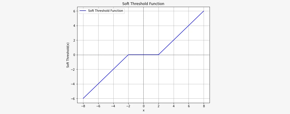
Calculating the subdifferential of the Lasso cost function and setting it equal to zero to find the minimum: $$0=\partial_{\beta_j} \left(RSS + L_1 \right)$$ $$0 = -\rho_j + \beta_j z_j + \partial_{\beta_j} \lambda ||\beta_j||$$ $$ \begin{equation} 0= \begin{cases} \ -\rho_j + \beta_j z_j - \lambda \ & \text{if}\ \beta_j < 0 \\ [ -\rho_j- \lambda , -\rho_j + \lambda ] & \text{if}\ \beta_j = 0 \\ \ -\rho_j + \beta_j z_j + \lambda \ & \text{if}\ \beta_j > 0 \end{cases} \end{equation} $$ We must be sure that the closed interval contains the zero. Hence $$- \lambda \leq \rho_j \leq \lambda$$ Solving for \(\beta_j\) we obtain: $$ \begin{aligned} \begin{cases} \beta_j = \frac{\rho_j + \lambda}{z_j} & \text{for} \ \rho_j < - \lambda \\ \beta_j = 0 & \text{for} \ - \lambda \leq \rho_j \leq \lambda \\ \beta_j = \frac{\rho_j - \lambda}{z_j} & \text{for} \ \rho_j > \lambda \end{cases} \end{aligned} $$ which we can express using the soft threshold function. $$ \begin{aligned} \frac{1}{z_j}S(\rho_j, \lambda)= \begin{cases} \beta_j = \rho_j + \lambda & \text{for} \ \rho_j < - \lambda \\ \beta_j = 0 & \text{for} \ - \lambda \leq \rho_j \leq \lambda \\ \beta_j = \rho_j - \lambda & \text{for} \ \rho_j > \lambda \end{cases} \end{aligned} $$ Here you can see how the soft thresholding function looks like:



So, in each step of coordinate descent, we need to update the parameters according to the formula: \(\frac{1}{z_j}\beta_j = S(\rho_j, \lambda)\)

Example - step by step implementation of LASSO

Time for some practical exercises - we'll implement LASSO!
As usual on this blog, we'll aim for simplicity and understanding of the algorithm, so we'll use simple functions instead of encapsulating the model in a python class.

Before, note that the term \(\rho_j\) can be rewritten to simplify the implementation (because our model has the form \(\hat{y}=\sum_{j=1}^{p}\beta_jX_j\)) $$\rho_j = \sum_{i=1}^{n}x_{ij} \left( y_i-\sum_{k\neq j}\beta_kx_{ik}\right) = \sum_{i=1}^{n}x_{ij} \left( y_i-\hat{y}_i+\beta_j x_{ij}\right)$$
To start with, let's remind ourselves of the steps of the coordinate descent algorithm for our particular case.

(1) Let's initialize the parameters of the method randomly.
(2) For specified number of iterations do:
\(\hspace{8mm}\) (2.1) For \(j=0,1,...,p\) (for all predictors = for all columns in dataset):
\(\hspace{16mm}\) (2.1.1) Compute:
$$\rho_j = \sum_{i=1}^{n}x_{ij} \left( y_i-\hat{y}_i+\beta_j x_{ij}\right)$$ \(\hspace{16mm}\) (2.1.2) Update parameters. Set:
$$\beta_j=S(\rho, \lambda)$$
In this example, we will use the same data that we used in the article about ridge regression: (From Theory to Practice: Ridge Regression for Improved Predictive Models).

import numpy as np

X = np.array([[0.8,  1.2,  0.5,  -0.7, 1.0],
              [1.0,  0.8,  -0.4, 0.5,  -1.2],
              [-0.5, 0.3,  1.2,  0.9,  -0.1],
              [0.2,  -0.9, -0.7, 1.1,  0.5]])

y = np.array([3.2, 2.5, 1.8, 2.9])

Similar to ridge regression, before building the model, we need to standardize the data so that the mean is zero and the variance is 1.

X = (X-X.mean(axis=0))/X.std(axis=0)

Before we start building the model, we also need to determine the hyperparameter \(\lambda\) responsible for regularization.

LAMBDA = 0.1

Before we implement the coordinate descent algorithm, which will allow us to update the model parameters, let's define the soft threshold function that we will use in our coordinate descent algorithm.

def soft_threshold(rho, lamda):
    if rho < - lamda:
        return (rho + lamda)
    elif rho >  lamda:
        return (rho - lamda)
    else: 
        return 0

That was simple. Now for the more complicated part, the coordinate descent algorithm.
This time, let's first demonstrate the whole function and then explain step by step what is happening there.

def coordinate_descent_lasso(X, y, lamda, max_iter=1000):
    n_features = X.shape[1] # number od predictors in our dataset
    beta = np.random.uniform(-1,1,n_features) # initialize random parameters
    for iteration in range(max_iter):
        for j in range(n_features):
            X_j = X[:,j]
            r_j = (X_j * (y - np.dot(X, beta) + beta[j] * X_j)).sum()
            beta[j] = soft_threshold(r_j, lamda) / (X_j ** 2).sum()
    return beta

Our function takes four arguments:
• \(\texttt{X}\) - matrix with predictors,
• \(\texttt{y}\) - target variable,
• \(\texttt{lamda}\) - the regularization parameter (in python lambda is a keyword for lambda function, but this time let it be)
• \(\texttt{max_iter}\) - the maximum number of iterations, with a default value of 1000

Then, we define number of features (predictors) in the dataset by accessing the second dimension of the feature matrix. We also need to initialize \(\texttt{beta}\) vector with all parameters we want to estimate (\(\beta_1,...,\beta_p\)). We initialize parameter vector with random values sampled from a uniform distribution between -1 and 1. The length of beta is equal to the number of features in the dataset.

The first loop iterates over \(\texttt{max_iter}\) a specified number of iterations. Sometimes additionally, the convergence criterion is implemented.

Within each iteration, there is another loop that iterates over each feature (predictor) in the dataset.
For each feature we calculate residuals (\(\texttt{r_j}\)) using the formula: $$\rho_j = \sum_{i=1}^{n}x_{ij} \left( y_i-\hat{y}_i+\beta_j x_{ij}\right)$$ Then we update the \(j\)-th parameter (\(\texttt{beta[j]}\)) using the soft thresholding function. It divides by \(z_j\), the result by the sum of squares of the \(j\)-th column of \(X\).
Finally, our function returns the updated parameter vector beta after the specified number of iterations.

That's all! Simpler than it might have seemed at first! The entire implementation of the key coordinate descent algorithm for LASSO took us only 10 lines of code!

At the end, as usual, we provide the entire code.

import numpy as np

def soft_threshold(rho, lamda):
    if rho < - lamda:
        return (rho + lamda)
    elif rho >  lamda:
        return (rho - lamda)
    else: 
        return 0

def coordinate_descent_lasso(X, y, lamda, max_iter=1000):
    n_features = X.shape[1] # number od predictors in our dataset
    beta = np.random.uniform(-1,1,n_features) # initialize random parameters
    for iteration in range(max_iter):
        for j in range(n_features):
            X_j = X[:,j]
            r_j = (X_j * (y - np.dot(X, beta) + beta[j] * X_j)).sum()
            beta[j] = soft_threshold(r_j, lamda) / (X_j ** 2).sum()
    return beta

# Example usage:
# Generate some random data
X = np.array([[0.8,1.2,0.5,-0.7,1.0],
[1.0,0.8,-0.4,0.5,-1.2],
[-0.5,0.3,1.2,0.9,-0.1],
[0.2,-0.9,-0.7,1.1,0.5]])

# scale
X = (X-X.mean(axis=0))/X.std(axis=0)

y = np.array([3.2, 2.5, 1.8, 2.9])

# Set regularization parameter
LAMBDA = 0.1

# Run coordinate descent
beta_lasso = coordinate_descent_lasso(X, y, lamda=LAMBDA, max_iter=1000)
print("Estimated beta:", beta_lasso)

Feature selection with \(\lambda\)

We mentioned that LASSO has the property of predictor selection. This is because as lambda increases, the regularization penalty starts pulling the coefficients β towards zero, automatically imposing predictor selection. The image below illustrates this relationship.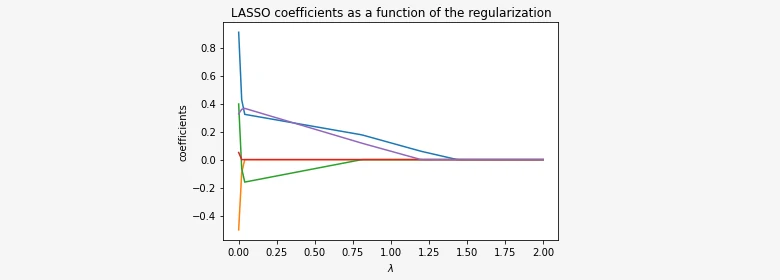


If we choose \(\lambda=1\), only the purple and blue lines don't intersect the OX axis. The remaining lines, red, green, and orange, align with the OY axis, indicating that these three coefficients have been shrinked to zero. Thus, these three variables have no influence on the model and can be removed from it. That's why we say LASSO imposes feature selection.

Conclusion:

In this blog post, we explored the concept of LASSO regression, a flexible technique in regression analysis particularly beneficial in scenarios where selecting features and achieving sparsity are essential. Through its regularization term, LASSO regression effectively manages the trade-off between model complexity and predictive accuracy.

We outlined the fundamental steps involved in LASSO regression, spanning from data normalization to the iterative coordinate descent algorithm for parameter estimation. Using clear examples and explanations, we showcased LASSO regression's capability to handle high-dimensional data and encourage sparse solutions by shrinking coefficients towards zero.

In summary, LASSO regression provides a robust approach to feature selection and regularization in linear regression models, proving indispensable for addressing real-world regression challenges across diverse domains. By understanding its principles and applications, practitioners can leverage LASSO regression to construct more interpretable and predictive models that excel in scenarios involving high-dimensional data and intricate feature relationships.

Happy coding! 😁