t-SNE: Visualizing Multidimensional World in 2D

---

Some time ago, we learned about PCA — one of the most popular dimensionality reduction algorithms. It enables us to reduce the number of features in a dataset in a simple and efficient way while retaining as much information as possible.
PCA is a linear method, meaning it performs well in representing data where relationships between features are linear. However, for more complex datasets - such as images, text, or biological data - linearity may be insufficient to capture meaningful relationships. In such cases, we need a more advanced approach. One such algorithm is t-SNE.

Understand the context

The t-SNE algorithm, or more precisely, t-Distributed Stochastic Neighbor Embedding, whose principles we will explain in this article, is not, contrary to appearances, a competing method to the well-known Principal Component Analysis (PCA).
While it can be said that the goal of t-SNE — dimensionality reduction - is essentially the same as that of PCA, the way these algorithms achieve this goal makes them fundamentally different and gives them completely distinct properties, leading to entirely different applications. This is precisely why it's worth learning about t-SNE - it expands our toolkit for applying algorithms in practice.

Before diving into the specifics and detailing how the t-SNE algorithm works, let’s first explore its historical background and the circumstances of its creation.

SNE - a close relative of t-SNE

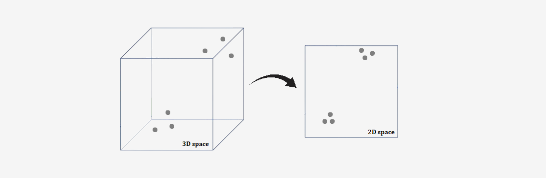
To be honest, the t-SNE algorithm is not an entirely original idea, but rather an improvement on another method. The history of the t-SNE algorithm begins with an earlier approach called Stochastic Neighbor Embedding (SNE), developed by Geoffrey Hinton and Sam Roweis in 2002.

The main idea behind SNE was to create an algorithm that enables mapping high-dimensional data into a lower-dimensional space while preserving the local relationships between points.
SNE worked by trying to preserve information about which points in the data are close to each other. First, in the original high-dimensional space, it calculats the probability that two points are neighbors — the closer they are to each other, the higher the probability. Then, the algorithm tries to recreate these same relationships in a lower-dimensional space (using the concept of information theory, specifically Kullback-Leibler divergence).
To achieve this, it checked how much the neighborhood relationships between the original and new space differed. The algorithm then adjusted the positions of the points in the lower-dimensional space so that these differences were minimized. This way, new, simplified data was obtained that preserved the local similarities from the original set.

But, SNE had significant limitations:
• The algorithm tended to collapse points in the target space, making it difficult to distinguish clusters.
• Using a Gaussian distribution in the target space led to difficulties in capturing appropriate relationships between distant points.

In 2008, Laurens van der Maaten and Geoffrey Hinton proposed an improved version of SNE — the t-Distributed Stochastic Neighbor Embedding algorithm. This was in response to the issues of the original SNE.

But more on that in a moment. Let's start with the original version, the SNE method.

SNE - Stochastic Neighbor Embedding

The first step in the SNE algorithm is to calculate the probability that two points in the high-dimensional space are neighbors. This probability depends on their distance: the closer two points are, the higher the probability that they will be considered neighbors.

After calculating the probabilities for the points in the high-dimensional space, the SNE algorithm tries to reproduce these same probabilities in a lower-dimensional space (e.g., 2D or 3D). The goal is for points that were close to each other in the high-dimensional space to also be close to each other in the low-dimensional space, and for points that were far apart to remain separated. To adjust the positions of the points in the low-dimensional space, the algorithm uses a cost function known as the Kullback-Leibler (KL) divergence, which measures the difference between two probability distributions. The goal is to minimize this divergence — that is, to match the probability distributions from the high-dimensional space to those in the low-dimensional space. Optimization involves adjusting the positions of the points in the low-dimensional space so that the differences between the neighborhood probabilities in both spaces are as small as possible. The algorithm changes the positions of the points until the KL divergence is minimized.
That's basically it! Now, let's move on to the details.

How to convert distances into probabilities?

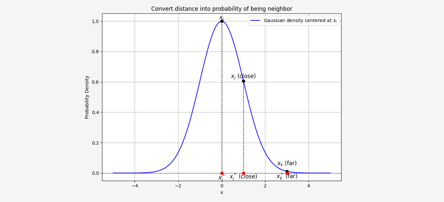
In the first step of the SNE algorithm, we need to convert distances into probabilities of being neighbors. How can we do this? Using conditional probability!

Let’s say we want to define \( p_{j|i} \), which represents the probability that point \( x_i \) would choose point \( x_j \) as its neighbor. This probability is determined based on the distance between the two points.
We can define this conditional probability using a Gaussian distribution centered at \( x_i \), where the probability of \( x_j \) being a neighbor of \( x_i \) depends on the distance between \( x_i \) and \( x_j \).
Let us recall how the density function is described for the Gaussian distribution. $$ f(x) = \frac{1}{\sqrt{2\pi\sigma^2}} \exp \left( -\frac{(x - \mu)^2}{2\sigma^2} \right) $$ So, conditional probability is given by (part \(\frac{1}{\sqrt{2\pi\sigma^2}}\) simplifies because it appears both in the numerator and the denominator): $$ p_{j|i} = \frac{\exp\left(-\frac{||x_i - x_j||^2}{2\sigma_i^2}\right)}{\sum_{k \neq i} \exp\left(-\frac{||x_i - x_k||^2}{2\sigma_i^2}\right)} $$ Where:
• \( ||x_i - x_j||^2 \) is the squared Euclidean distance between the points \( x_i \) and \( x_j \)
• \( \sigma_i^2 \) is a variance parameter that controls the spread of the distribution, determining how tight the neighbors are around \( x_i \)
The denominator normalizes the probability so that the sum of the probabilities for all neighbors of \( x_i \) equals 1.

This formula ensures that the closer a point \( x_j \) is to \( x_i \), the higher the probability \( p_{j|i} \) will be. We can ilustrate this on plot below: The next step is to similarly compute the probabilities \( p_{i|j} \) for the reverse case, where \( x_j \) chooses \( x_i \) as its neighbor. But why is this necessary?
After all, it doesn't matter whether we measure the distance from \( x_i \) to \( x_j \) or vice versa - the distance is always the same. Unfortunately, the value of the parameter \( \sigma_i \) may differ for each point, which means that the measure \( p_{j|i} \) is not symmetric, and in general, \( p_{j|i} \neq p_{i|j} \).
The fact that these probabilities are not symmetric is one of the major drawbacks of the SNE algorithm, which is addressed in the t-SNE version. The issue of asymmetry in the conditional probabilities makes what is called the crowding problem a real challenge.
The way in which the values of \( \sigma_i \) are determined could be the subject of a separate article. For now, let’s assume that they can be obtained through certain experiments — which we will discuss later.

Anyway, we now have a way to transform the distances between points into probabilities in high dimensional space. Now we need to do this for the low-dimensional space. However, it won’t be done in exactly the same way.

For the low-dimensional counterparts \( y_i \) and \( y_j \) of the high-dimensional data points \( x_i \) and \( x_j \), it is possible to compute a similar conditional probability, which we denote by \( q_{j|i} \).
In the low-dimensional space, we also use Gaussian neighborhoods, but with a fixed variance. Let’s set this variance to \( 1/2 \), which simplifies the formula to: $$ q_{j|i}=\frac{\exp(-||y_i-y_j||^2)}{\sum_{k \neq i}\exp(-||y_i-y_k||^2)} $$ The formula above describes the probability that the point \( y_i \), mapped in the low-dimensional space, will choose point \( y_j \) as its neighbor.

If the points in the low-dimensional space \( y_i \in \mathcal{Y} \) perfectly modeled the similarities between points in the high-dimensional space \( x_i \in \mathcal{X} \), the conditional probabilities \( p_{j|i} \) and \( q_{j|i} \) would be equal.
Unfortunately, perfect matching is usually not possible — but that’s okay! Striving for perfection is enough. The entire challenge of the SNE algorithm lies in finding a low-dimensional representation of the data that minimizes the mismatch (strives for perfection) between \( p_{j|i} \) and \( q_{j|i} \).

Embedding

In machine learning, we often encounter the problem of mapping a high-dimensional space to a low-dimensional space. This process is called embedding.

Embedding
An embedding is an injective mapping \( f: \mathcal{X} \to \mathcal{Y} \) of object \( \mathcal{X} \) into object \( \mathcal{Y} \) that preserves the properties of the embedded object (the specific properties preserved depend on the theory being considered).

In the context of machine learning, embedding refers to the process of mapping high-dimensional data into a lower-dimensional space while preserving essential information, such as similarities or relationships between data points.

Formally, an embedding is a function \( f: \mathcal{X} \to \mathcal{Y} \), where:
• \( \mathcal{X} \subseteq \mathbb{R}^D \) - High-dimensional input space (with \( D \) dimensions).
• \( \mathcal{Y} \subseteq \mathbb{R}^d \) - Low-dimensional target space (with \( d \ll D \)).

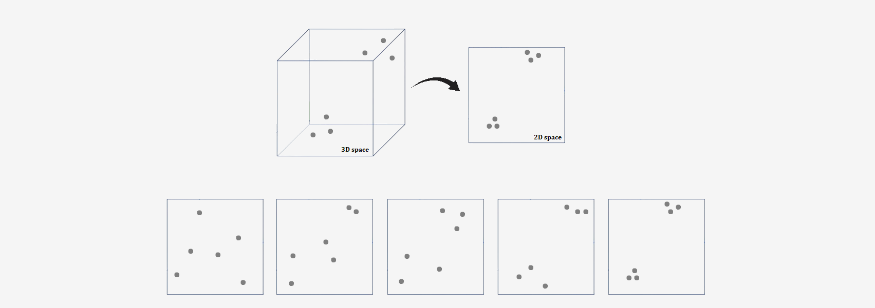
In fact, we can determine the dimensionality of our low-dimensional space ourselves. We decide how small the space we want to map our high-dimensional data onto should be. However, the t-SNE algorithm is typically used for visualizing high-dimensional data, and our limited ability to draw essentially ends at two dimensions. For this reason, t-SNE usually reduces the dimensionality to 2 dimensions, making it convenient to present the results in the form of a plot.

In our case, the goal is to find an embedding such that the distributions \( p_{j|i} \) and \( q_{j|i} \) are as similar as possible. We can also express this differently: to minimize the differences between the distributions \( p_{j|i} \) and \( q_{j|i} \).

But how do we measure the differences between two probability distributions, or more importantly, how do we quantify how much two probability distributions differ from each other?

Kullback-Leibler divergence

Ideally, we would have a tool that, when given two probability distributions, would return a number telling us how much these distributions differ. This is not trivial, but fortunately, there is a tool (though not perfect) used in information theory for comparing two distributions, called Kullback-Leibler divergence.

KL divergence is a measure that evaluates how one probability distribution differs from another. Intuitively, we can think of it this way:
How much are we wrong if we assume that both distributions are the same? or How much information do we lose if we use distribution \( p \) instead of \( q \)?

With the intuition in place, it's time for the formal definition.

Kullback-Leibler divergence
The Kullback-Leibler divergence for discrete probability distributions \( P \) and \( Q \) defined on the same sample space \( \mathcal{X} \) is given by: $$ D_{\text{KL}}(P \parallel Q) = \sum_{x \in \mathcal{X}} P(x) \ln \left( \frac{P(x)}{Q(x)} \right) $$

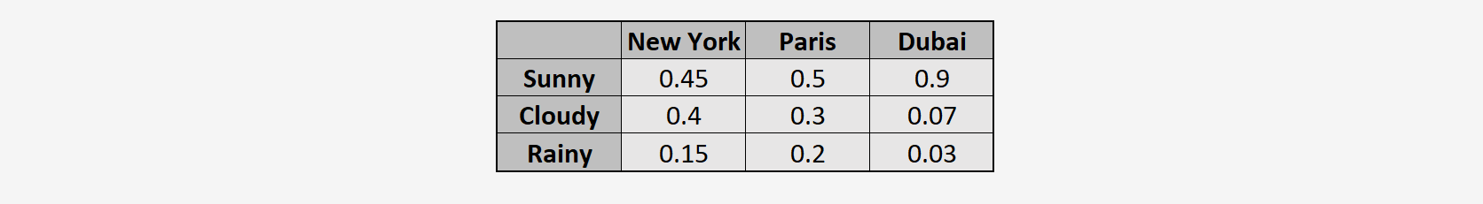Let's illustrate how KL divergence works with an example. Let's look at the weather distributions in 3 big cities. We'll use KL divergence to see how much the weather in New York differs from Paris and Dubai. Now, using the KL divergence formula, we compute how different is weather in New York and Paris: $$ D_{KL}(P_{\text{NY}} \parallel Q_{\text{Paris}}) = 0.45 \ln \left(\frac{0.45}{0.5}\right) + 0.4 \ln \left(\frac{0.4}{0.3}\right) + 0.15 \ln \left(\frac{0.15}{0.2}\right) = -0.0474 + 0.1151 -0.0432 = 0.0245 $$ Now, how different is weather in New York and Dubai: $$ D_{KL}(P_{\text{NY}} \parallel Q_{\text{Dubai}}) = 0.45 \ln \left(\frac{0.45}{0.9}\right) + 0.4 \ln \left(\frac{0.4}{0.07}\right) + 0.15 \ln \left(\frac{0.15}{0.03}\right) = -0.3119 + 0.6972 + 0.2414 = 0.6267 $$ We can see that the value of the KL divergence is very small for \(D_{KL}(P_{\text{NY}} \parallel Q_{\text{Paris}})\) and significantly higher for \(D_{KL}(P_{\text{NY}} \parallel Q_{\text{Dubai}})\). From this, we can infer that the weather in New York is much more similar to that in Paris than to that in Dubai.


Since we have already spent some time discussing KL divergence, it’s worth pausing for a moment to point out a particular property of this measure that might keep you up at night - Kullback-Leibler divergence is not symmetric!

This means that the difference between two probability distributions depends on which distribution you are comparing with which. This might be a bit surprising at first and seem counterintuitive, but it has its pros and cons.
One of the main disadvantages is that it cannot be directly interpreted as a measure of the difference between two distributions. You might be thinking, "What?! We are using it precisely because it’s supposed to measure the differences between distributions!" The truth is, that’s not exactly our goal. Indeed, the fact that we can choose the direction of comparison is an advantage!

In the SNE algorithm, the goal is to find a low-dimensional representation of points in space that best preserves the local relationships in the high-dimensional space. In this case, the asymmetry of KL divergence is actually desirable. We cannot change the probability distribution for the high-dimensional space - it is determined by the dataset. However, in the low-dimensional space, we choose where the points should be placed, so we can change their distribution. In summary, we do not care about making these distributions interchangeable. Instead, we aim to approximate the neighborhood probabilities in the low-dimensional space to those from the high-dimensional space.

Let's return to our discussion.

SNE - how to find low-dimensional space?

We know how to transform the distances between points into probabilities. These probabilities, for all the points in our dataset, together form a probability distribution. Since we have two spaces - one high-dimensional and the other low-dimensional - we have two probability distributions defined by \( p_{j|i} \) and \( q_{j|i} \). We have just learned how to measure the difference between two distributions.
We want to map the original high-dimensional space into a low-dimensional one without losing information, meaning we want the two distributions, \( p_{j|i} \) and \( q_{j|i} \), to differ as little as possible.
This is achieved by minimizing a cost function, which is the sum of Kullback-Leibler divergences between the original (\( p_{j|i} \)) and induced (\( q_{j|i} \)) distributions over neighbors for each observation: $$ C = \sum_{i}D_{KL}(P_i||Q_i) = \sum_i\sum_j p_{j|i} \ln\left(\frac{p_{j|i}}{q_{j|i}}\right) $$ Since the cost function is quite complicated, finding its minimum analytically would be a significant challenge (in fact, it doesn't have an analytical solution). In such cases, we use iterative methods, just as we did in the case of logistic regression. In this case, we will use one of the simplest methods, gradient descent.

Gradient Descent
The gradient descent method is an iterative algorithm for finding the minimum of a given objective function \( f \): $$ f : D \mapsto \mathbb{R}$$ where \( D \subset \mathbb{R}^n \).

The assumptions for the method are as follows:
• \( f \in \mathrm{C}^1 \) (the function is differentiable and has continuous derivative)
• \( f \) is strictly convex in the examined domain

Under these conditions, a local minimumcan be found by iteratively updating the current estimate of the minimum. Specifically, the algorithm uses the negative gradient of the function to guide the search towards the minimum.
In each iteration, the current point \( \mathbf{x}_t \) is updated using the rule:
\[ \mathbf{x}_{t+1} = \mathbf{x}_t - \eta \nabla f(\mathbf{x}_t) \] where:
• \( \mathbf{x}_t \) is the current point
• \( \eta \) is the learning rate (step size)
• \( \nabla f(\mathbf{x}_t) \) is the gradient of the function at \( \mathbf{x}_t \)

This process continues until convergence, where the gradient becomes small, indicating that a minimum has been reached.

Alright, we have a method that will help us optimize the cost function. Unfortunately, it requires finding its gradient. Unfortunately, this isn't the most pleasant computational part, and since it concerns the SNE algorithm and is just an introduction to the t-SNE method, we'll save you from the tedious calculations (though they will be present in the actual t-SNE version). The results, however, are surprisingly simple: $$\frac{\partial C}{\partial y_i} = 2\sum_j (p_{j|i} - q_{j|i} + p_{i|j} - q_{i|j})(y_i-y_j)$$ The gradient \( \frac{\partial C}{\partial y_i} \) represents the total force acting on each map point, where each spring adjusts the position of a point in the low-dimensional map in such a way that the local structure of the data is better preserved.
Imagine each pair of map points \( y_i \) and \( y_j \) is connected by a spring. The force that the spring applies is always along the line that connects these two points (the direction of \( y_i - y_j \)). The strength of this force depends on how far apart the two points are in the map.
The force exerted by the spring depends on the difference between the similarity in the high-dimensional space (represented by \( p_{j|i} \) and \( p_{i|j} \)) and the similarity in the low-dimensional space (represented by \( q_{j|i} \) and \( q_{i|j} \)). The strength of the force depends on how well the distances between the map points match the similarities of the original, high-dimensional data points. If the points are too far apart or too close in the map compared to the high-dimensional space, the spring will either pull the points together or push them apart. This difference between the high-dimensional similarities (how close the points should be) and the map's current representation is what determines the stiffness of the spring, meaning how strongly it wants to change the positions of the points.


By moving in the direction opposite to the gradient, we can get closer to the local minimum of our cost function in each iteration of gradient descent algorithm. $$y_i^{(t)}= y_i^{(t-1)} - \eta \frac{\partial C}{\partial y_i}$$
Although the gradient of the cost function has a nice physical interpretation, it is computationally expensive to obtain. Furthermore, our solution is affected by the crowding problem. In the next section, we will show how these issues can be addressed.

Symmetric SNE

Symmetric SNE is an improved version of the SNE algorithm that introduces symmetry into the probability calculations, improving the quality and stability of the optimization process.

As an alternative to minimizing the sum of Kullback-Leibler divergences between the conditional probabilities \(p_{j|i}\) and \(q_{j|i}\), it is also possible to minimize a single Kullback-Leibler divergence between the joint probability distribution \(P\) in the high-dimensional space and the joint probability distribution \(Q\) in the low-dimensional space: $$C = D_{\text{KL}}(P \parallel Q) = \sum_i \sum_j p_{ij} \ln \left( \frac{p_{ij}}{q_{ij}} \right)$$ Similarly, pairwise similarities in the high-dimensional space \(p_{ij}\) could be defined as: $$p_{ij}=\frac{\exp\left(-\frac{||x_i-x_j||^2}{2\sigma_i^2}\right)}{\sum_{k \neq l}\exp\left(-\frac{||x_k-x_l||^2}{2\sigma_i^2}\right)}$$ In classical SNE, the probabilities are asymmetric - different values of \(p_{j|i}\) and \(p_{i|j}\) are calculated for each point, which leads to issues in representing relationships between points in the low-dimensional space. In symmetric SNE, the probabilities are symmetric, meaning that we treat \(p_{j|i}\) and \(p_{i|j}\) in the same way, which results in a more consistent mapping of points. This allows the method to better reflect the mutual relationships between points.

Unfortunately, this definition creates a problem when \(x_i\) is an outlier (all distances \(||x_i - x_j||^2\) are large for \(x_i\)). For such observations, the values of \(p_{ij}\) are extremely small for each \(j\), so their location in the low-dimensional space after transformation to \(y_i\) has very little impact on the cost function. We avoid this issue by defining the joint probabilities \(p_{ij}\) in the high-dimensional space as symmetric conditional probabilities, meaning: $$p_{ij}=\frac{p_{j|i}+p_{i|j}}{2n}$$ This ensures that \(\sum_{j} p_{ij} > \frac{1}{2n}\) for all points \(x_i\), so each data point \(x_i\) contributes significantly to the cost function.

The main advantage of the symmetric version of SNE is the simpler form of its gradient, which is faster to compute: $$\frac{\partial C}{\partial y_i} = 4\sum_j (p_{ij}-q_{ij})(y_i-y_j)$$ Although SNE performs quite well, still it has some drawbacks that I mentioned in earlier sections of this article. One of them is the crowding problem. In the next section, we will present an improvement to the SNE method introduced a few years later, called t-Distributed Stochastic Neighbor Embedding (t-SNE) which aims to mitigate these problems.

t-Distributed SNE (t-SNE)

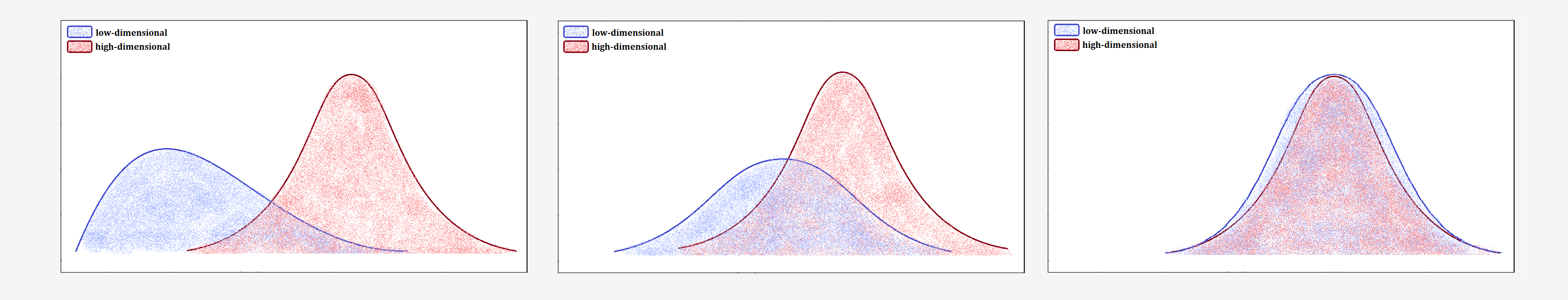
The crowding problem refers to the difficulty of accurately representing distances between points that are moderately distant in high-dimensional space when projected into low-dimensional space. As a result, these points are often placed too close to each other, leading to distortions in the low-dimensional representation.
Imagine you have data from different clusters that are far apart in high-dimensional space. When you try to map them onto a plane, it becomes challenging to preserve those large distances. The clusters are squeezed together, making the differences between them less visible.

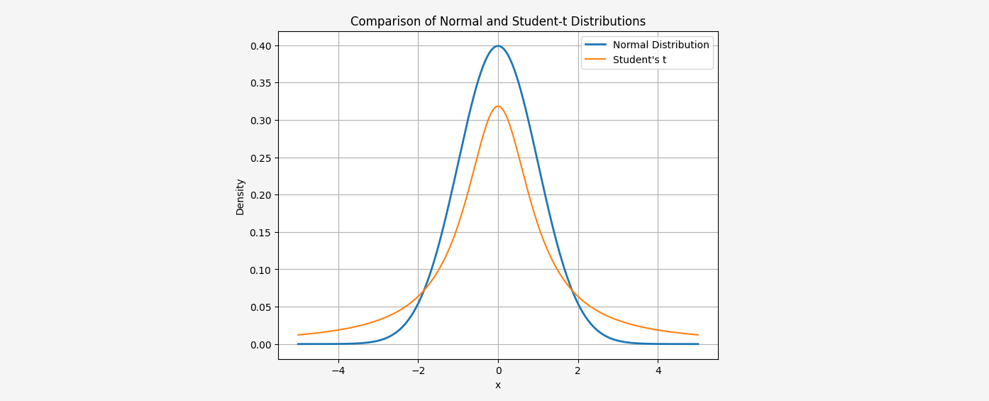
To address this issue, t-SNE uses a Student-t distribution with one degree of freedom to transform distances in low-dimensional space into probabilities. The Student-t distribution has heavier tails than the Gaussian distribution, allowing for better representation of moderate distances in high-dimensional space as larger distances on the map.
The normal distribution used in SNE decreases rapidly for large distances. In practice, this means that if two points are far apart, the difference between them in low-dimensional space becomes irrelevant. The Student-t distribution’s heavier tails ensure that even for large distances, the probability does not decrease as sharply. In t-SNE, we use the Student’s t-distribution with one degree of freedom, where the joint probability distribution \( q_{ij} \) is defined as: $$q_{ij}=\frac{(1+||y_i-y_j||^2)^{-1}}{\sum_{k \neq l}(1+||y_k-y_l||^2)^{-1}}$$ Notice that in t-SNE, we only change the distribution in the low-dimensional space, leaving the distribution in the high-dimensional space unchanged. This allows us to focus on adjusting the map to best capture local and moderate relationships between points, while simultaneously eliminating the crowding problem.

In t-SNE, we changed the distribution used to convert distances into probabilities. All other assumptions remain essentially the same. We optimize the same cost function as in Symmetric SNE: $$C = D_{\text{KL}}(P \parallel Q) = \sum_i \sum_j p_{ij} \ln \left( \frac{p_{ij}}{q_{ij}} \right)$$ whose gradient is as follows: $$\frac{\partial C}{\partial y_i} = 4\sum_j (p_{ij}-q_{ij})(y_i-y_j)(1+||y_i-y_j||^2)^{-1}$$ How did we derive this gradient? This requires tedious calculations, which I promised to include.

At the beginning, let's introduce the following notation: $$ E_{ij} := 1 + ||y_i - y_j||^2 $$ $$ Z := \sum_{k,l \neq k} (1 + ||y_k - y_l||^2)^{-1} = \sum_{k,l \neq k} E_{kl}^{-1} $$ Note that: $$ q_{ij} = \frac{(1 + ||y_i - y_j||^2)^{-1}}{\sum_{k,l \neq k} (1 + ||y_k - y_l||^2)^{-1}} = \frac{E_{ij}^{-1}}{Z} $$ The cost function can be defined as: $$ C = \sum_{k,l \neq k} p_{lk} \ln \left( \frac{p_{lk}}{q_{lk}} \right) $$ But using the property of logarithms \( \log\left(\frac{x}{y}\right) = \log(x) - \log(y) \), we can split this into two parts: $$ C = \sum_{k,l \neq k} p_{lk} \ln p_{lk} - p_{lk} \ln q_{lk} $$ Again, using the same property of the logarithm and the adopted notation, we can write: $$ C = \sum_{k,l \neq k} p_{lk} \ln p_{lk} - p_{lk} \ln E^{-1}_{kl} + p_{lk} \ln Z $$ Now, we will compute the derivative of the cost function with respect to \( y_i \). Notice immediately that the first part does not depend on \( y_i \), so it will cancel out after differentiation. $$ \frac{\partial C}{\partial y_i} = \underbrace{\sum_{k,l \neq k} - p_{lk} \frac{\partial}{\partial y_i} \left[ \ln E^{-1}_{kl} \right]}_{\text{part I}} + \underbrace{\sum_{k,l \neq k} p_{lk} \frac{\partial}{\partial y_i} \left[ \ln Z \right]}_{\text{part II}} $$ We start with the first term, noting that the derivative is non-zero when \(\forall j\), \(k = i\) or \(l = i\), that \(p_{ij} = p_{ij}\) and \(E_{ji} = E_{ij}\). $$ \text{[I]} = \sum_{k,l \neq k} - p_{lk} \frac{\partial}{\partial y_i} \left[ \ln E^{-1}_{kl} \right] = -2 \sum_{j\neq i} p_{ij} \frac{\partial}{\partial y_i} \left[ \ln E^{-1}_{ij} \right] $$ Let's focus on \(\frac{\partial}{\partial y_i} \left[ \ln E^{-1}_{ij} \right]\) $$ \frac{\partial}{\partial y_i} \left[ \ln E^{-1}_{ij} \right] = \frac{1}{(1 + ||y_i - y_j||^2)^{-1}}(-2(y_i-y_j)) = -2(y_i-y_j)E_{ij}^{-1} $$ Substituting, we get:: $$ \text{[I]} = -2 \sum_{j\neq i} p_{ij} \frac{\partial}{\partial y_i} \left[ \ln E^{-1}_{ij} \right] = 4 \sum_{j\neq i} p_{ij} E^{-1}_{ij} (y_i-y_j) $$ Now the second term. Using the fact that \( \sum_{k,l \neq k} p_{kl} = 1\) and that \( Z \) does not depend on \( k \) or \( l \) $$ \text{[II]} = \sum_{k,l \neq k} p_{lk} \frac{\partial}{\partial y_i} \left[ \ln Z \right] = \frac{1}{Z} \sum_{k', 'l\neq k'} \frac{\partial}{\partial y_i} E_{kl}^{-1} = 2 \sum_{j\neq i} -2 \frac{1}{Z} E_{ij}^{-2} (y_i-y_j) = -4 \sum_{j\neq i} q_{ij} E_{ij}^{-1} (y_i-y_j) $$ Hence, $$ \frac{\partial C}{\partial y_i} = 4 \sum_{j\neq i} p_{ij} E^{-1}_{ij} (y_i-y_j) - 4 \sum_{j\neq i} q_{ij} E_{ij}^{-1} (y_i-y_j) $$ Factoring out \( E^{-1}_{ij} (y_i - y_j) \) and returning to the original notation, we ultimately obtain: $$ \frac{\partial C}{\partial y_i} = 4\sum_{j\neq i} (p_{ij}-q_{ij})(y_i-y_j)(1+||y_i-y_j||^2)^{-1} $$ Done! We now understand where this form of the gradient comes from. We could now use gradient descent to find the best arrangement of points in the low-dimensional space. However, the authors of the original paper propose an improved version of gradient descent that uses a momentum term to reduce the number of required iterations — or, colloquially speaking, to speed up the algorithm.

The formula that allows the algorithm to approach the local minimum with each iteration is: $$ y_i^{(t)} = y_i^{(t-1)} - \eta \frac{\partial C}{\partial y_i} + \alpha(t-1) \left( y_i^{(t-1)} - y_i^{(t-2)} \right) $$ where \(\eta\) is the learning rate, and \(\alpha(t)\) is the momentum at time \(t\).

This procedure works best when the momentum term is small until the map points become well-organized. In the original paper, the authors chose the following momentum schedule for their algorithm results: $$ \alpha(t) = \left\{ \begin{array}{ll} 0.5 & \mbox{if } t < 250 \\ 0.8 & \mbox{otherwise } \end{array} \right. $$ We already have a general idea of how the t-SNE method works and how to find the best arrangement of points in a lower-dimensional space. However, we haven't yet mentioned one quite important issue.

Perplexity

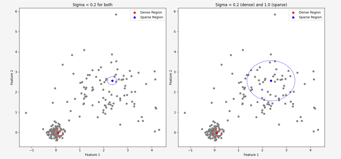
At the very beginning of our article, when we attempted to convert distances between points into a probability distribution, we used a Gaussian distribution \(\mathcal{N}(\mu, \sigma^2)\) for this purpose. This distribution has two parameters: the mean and the variance. The mean represents the location of the point in space because we centered the distribution to be located at the given point. The variance, on the other hand, determines how tight the neighbors are around the point, but how to find \( \sigma\), separately for each point in the dataset!?

The simplest approach would be to use a single common value for all points, but it is highly unlikely that this would be a good choice, because the data density is usually not uniform throughout the dataset, so this idea is doomed to failure from the start.

In dense regions, where data points are close to each other, we would prefer to have a smaller value for the \(\sigma\) parameter to avoid considering points that are far apart as neighbors. In regions where the data points are not as close to each other, we would like to increase the \(\sigma\) value to capture some neighbors at all.
Before we proceed, it will be necessary to understand the definition of entropy. We have already mentioned entropy in other articles, but now we will need a more formal definition.

Entropy (Shannon entropy)
Let \( X \) be a random variable with values \( x_1, x_2, \dots, x_n \), occurring with probabilities \( p(x_1), p(x_2), \dots, p(x_n) \). The entropy is defined as the expected value of the logarithm of the inverse of the probability of an event: $$ \mathrm{H}(X) = \mathbb{E}[-\log_2 p(X)] = - \sum_{i=1}^{n} p(x_i) \log_2 p(x_i) $$
Note:
The base of the logarithm can be different from 2, in which case only the unit in which we express entropy changes. In information theory, the logarithm with base 2 is most commonly used, in which case the unit of entropy is a bit. For \( e \) as the base, this unit is called a nat.

The entire idea of how to universally find the values of the parameters \( \sigma_i \) is based on Shannon entropy. The entropy of a probability distribution is a measure of the uncertainty of that distribution. The more spread out the distribution is (for example, for a large \( \sigma_i \)), the more dispersed the probabilities assigned to different points are. This means that as \( \sigma_i \) increases, the distribution \( P_i \) becomes flatter (higher entropy), and more points can be considered as neighbors of a given point. We can understand it this way: When a larger number of points is considered as potential neighbors, the uncertainty in determining which points are the closest increases.

From a mathematical perspective, entropy \( H(P) \) is a logarithm with base 2, meaning it tells us how many bits of information are needed to encode the outcomes of a given distribution. When we consider \( 2^{H(P)} \), we obtain the number of possible outcomes the model can consider, treating entropy as a measure of the size of this outcome space.
For example, if the entropy is 3, it means there are 8 possible outcomes (since \( 2^3 = 8 \)).

This transformation makes it easier to interpret entropy in the context of the number of possible states included in the distribution. This allows us to better understand how complex the distribution is and how many different options need to be taken into account. Let us therefore define perplexity as: $$ \operatorname{Perp}(P_i) = 2^{H(P_i)} $$ where \(\mathrm{H}(P_i)\) is the Shannon entropy of \(P_i\) measured in bits $$ \mathrm{H}(P_i)=-\sum_j p_{j|i} \log_2 p_{j|i} $$ Perplexity can be interpreted as the number of possible neighbors that are considered in the distribution. The higher the perplexity, the more different points are considered as potential neighbors in the distribution. On the other hand, low perplexity means that the distribution only considers a few points as neighbors.

In t-SNE, we want to find values of \( \sigma_i \) for each point that give the appropriate perplexity value. We want each point \( i \) to have neighbors that are suitably close and represent cohesion in the low-dimensional space. To achieve this, t-SNE uses a binary search algorithm to adjust \( \sigma_i \) to ensure the desired perplexity value.
Once the perplexity is determined, the values of \( \sigma_i \) are optimized so that each point has the appropriate \( \sigma_i \) corresponding to the given perplexity. Through this process, the values of \( \sigma_i \) are adjusted to obtain a local, realistic representation of neighborhoods in the low-dimensional space.


Thanks to the introduction of perplexity, we no longer need to worry about how to estimate all the \( \sigma_i \) parameters separately for each data point. Instead, we only need to define one value - perplexity. We must also do this before running the algorithm. Therefore, perplexity is a hyperparameter of the t-SNE method.

We have significantly simplified the situation. We no longer have to specify hundreds of thousands of parameter values, just one. However, the question still remains: what value should we choose?
The authors of the original paper claim that "The performance of SNE is fairly robust to changes in the perplexity, and typical values are between 5 and 50." Unfortunately, there is no guarantee that values within this range will always yield good results, but it is usually a good starting point.

t-SNE algorithm

Let's summarize all the considerations so far with a simple set of instructions that implement the t-SNE algorithm:

t-SNE algorithm:

1. Calculate pairwise affinities \( p_{j|i} \) using the perplexity \( \text{Perp} \) $$ p_{j|i} = \frac{\exp\left(-\frac{||x_i - x_j||^2}{2\sigma_i^2}\right)}{\sum_{k \neq i} \exp\left(-\frac{||x_i - x_k||^2}{2\sigma_i^2}\right)} $$ then set $$ p_{ij} = \frac{p_{j|i} + p_{i|j}}{2n} $$
2. Sample initial solution \( Y^{(0)} = \{y_1, y_2, \dots, y_n\} \) from a normal distribution \( \mathcal{N}(0, 10^{-4}I) \)
3. Iterate for \( t = 1 \) to \( T \):
   1. Compute low-dimensional affinities $$ q_{ij}=\frac{(1+||y_i-y_j||^2)^{-1}}{\sum_{k \neq l}(1+||y_k-y_l||^2)^{-1}} $$
   2. Compute the gradient \( \frac{\partial C}{\partial Y} \): $$ \frac{\partial C}{\partial y_i} = 4\sum_{j\neq i} (p_{ij}-q_{ij})(y_i-y_j)(1+||y_i-y_j||^2)^{-1} $$
   3. Update the low-dimensional representation: $$ Y^{(t)} = Y^{(t-1)} + \eta \frac{\partial C}{\partial Y} + \alpha(t-1) \left( Y^{(t-1)} - Y^{(t-2)} \right) $$

Example

The algorithm requires many iterations of tedious calculations, so we will not illustrate everything and will make many simplifications. However, we will try to show the most important points of the algorithm using simple examples.

Let's assume that our dataset consists of 3 observations with the following coordinates: $$ x_1=(0,1,3) \hspace{5mm} x_2=(2,1,1) \hspace{5mm} x_3=(2,0,2) $$ Let's further assume that this is the third iteration of the algorithm, and we know the results from the previous two iterations (remember that at the very beginning, the coordinates of the points in the target low-dimensional space are drawn from a normal distribution).
Let: $$ Y^{(1)} = \begin{bmatrix} 2.5000 & -1.1000 \\ 0.4500 & -0.7500 \\ 0.3300 & -1.4500 \end{bmatrix} \hspace{5mm} Y^{(2)} = \begin{bmatrix} 2.6272 & -1.1431 \\ 0.4916 & -0.7610 \\ 0.3465 & -1.4710 \end{bmatrix} $$ Let's also assume that the binary search algorithm found the following values of \(\sigma_i\): $$ \sigma_1=1 \hspace{5mm} \sigma_2=2 \hspace{5mm} \sigma_3=1.5 $$ The first step of our algorithm is to find pairwise affinities. For example, let's calculate \( p_{2|3} \), which is the probability that point \( x_3 \) would choose point \( x_2 \) as its neighbor: $$ \begin{align} p_{2|3} &= \frac{\exp\left(-\frac{||x_3 - x_2||^2}{2\sigma_3^2}\right)}{\sum_{k \neq 3} \exp\left(-\frac{||x_3 - x_k||^2}{2\sigma_3^2}\right)}= \\ &= \frac{\exp\left(-\frac{||x_3 - x_2||^2}{2\sigma_3^2}\right)}{\exp\left(-\frac{||x_3 - x_1||^2}{2\sigma_3^2}\right) + \exp\left(-\frac{||x_3 - x_2||^2}{2\sigma_3^2}\right)} \\ &= \frac{\exp\left(-\frac{||(2,0,2) - (2,1,1)||^2}{2 \cdot (1.5)^2}\right)}{\exp\left(-\frac{||(2,0,2) - (0,1,3)||^2}{2\cdot (1.5)^2}\right) + \exp\left(-\frac{||(2,0,2) - (2,1,1)||^2}{2\cdot (1.5)^2}\right)} \approx 0.7085 \end{align} $$ Notice that \(p_{3|2} \neq p_{2|3}\) $$ p_{3|2} = \frac{\exp\left(-\frac{||x_2 - x_3||^2}{2\sigma_2^2}\right)}{\exp\left(-\frac{||x_2 - x_1||^2}{2\sigma_2^2}\right) + \exp\left(-\frac{||x_2 - x_3||^2}{2\sigma_2^2}\right)} \approx 0.6791 $$ Similarly, we need to calculate the probabilities for all other pairs of points.

In the next step, we enforce symmetry for these probabilities. We define the joint probabilities according to the following formula: $$ p_{ij} = \frac{p_{j|i} + p_{i|j}}{2n} $$ Hence, for example, \( p_{23} = p_{32} \): $$ p_{23}=p_{32}= \frac{p_{2|3} + p_{3|2}}{2 \cdot 3} = \frac{0.7085 + 0.6791}{6} = 0.2313 $$ Similarly, we calculate the joint probabilities for the remaining points.

Let's say that we are currently at step \( t = 2 \) of the algorithm. From the previous iteration, we obtained the following coordinates of the points in the 2-dimensional space: $$ Y^{(2)} = \begin{bmatrix} 2.6272 & -1.1431 \\ 0.4916 & -0.7610 \\ 0.3465 & -1.4710 \end{bmatrix} $$ Now we need to find the low-dimensional affinities, i.e., $$ q_{ij}=\frac{(1+||y_i-y_j||^2)^{-1}}{\sum_{k \neq l}(1+||y_k-y_l||^2)^{-1}} $$ For example let's calculate \(q_{23}\): $$ q_{23} = \frac{(1+||y_2-y_3||^2)^{-1}}{(1+||y_1-y_2||^2)^{-1}+1+||y_1-y_3||^2)^{-1}+1+||y_2-y_3||^2)^{-1}} \approx \frac{0.6556}{0.1752+0.1585+0.6556} = 0.6626 $$ Proceeding similarly for the remaining points, we obtain: $$q_{12} = \frac{0.1752}{0.9893} = 0.1772$$ $$q_{13} = \frac{0.1585}{0.9893} = 0.1602$$ $$q_{23} = \frac{0.6556}{0.9893} = 0.6626$$ The next step of the algorithm is gradient descent. We will want to update the weights in order to achieve a better arrangement of the points. The direction in which our results improve is determined by the gradient: $$ \frac{\partial C}{\partial y_i} = 4\sum_{j\neq i} (p_{ij}-q_{ij})(y_i-y_j)(1+||y_i-y_j||^2)^{-1} $$ Let's calculate, for example, the derivative of our cost function with respect to the second coordinate: $$ \begin{align} \frac{\partial C}{\partial y_2} &= 4 \sum_{j \neq 2} (p_{2j} - q_{2j})(y_2 - y_j)(1 + ||y_2 - y_j||^2)^{-1} = \\ &= 4 \left((p_{21} - q_{21})(y_2 - y_1)(1 + ||y_2 - y_1||^2)^{-1} + (p_{23} - q_{23})(y_2 - y_3)(1 + ||y_2 - y_3||^2)^{-1} \right) = \\ &= 4 \left(0.1228\cdot (−2.1356,0.3821)\cdot 0.1752 −0.2126\cdot (0.1451,0.7100)\cdot 0.6556 \right) = \\ &= 4 \cdot \left[ (-0.0459, 0.0082) + (-0.0202, -0.0988) \right] = \\ &= 4 \cdot (-0.0661, -0.0906) = \\ &= (-0.2644, -0.3624) \end{align} $$ When we do the same for the remaining points, we obtain: $$ \frac{\partial C}{\partial Y} = \begin{bmatrix} 0.3148 & -0.0140 \\ -0.2644 & -0.3624 \\ -0.0488 & 0.3764 \end{bmatrix} $$ We already know the gradient of our cost function. Therefore, the last step of this iteration of the algorithm is to update the coordinates of the points in the low-dimensional space.

We know from the previous iteration \( Y^{(1)} \): $$ Y^{(1)} = \begin{bmatrix} 2.5000 & -1.1000 \\ 0.4500 & -0.7500 \\ 0.3300 & -1.4500 \end{bmatrix} $$ For this iteration, let's assume the learning rate is \( \eta = 0.2 \) and \( \alpha(t-1) = 0.5 \).

The coordinates are updated according to the formula: \[ Y^{(3)} = Y^{(2)} + 0.2 \cdot \frac{\partial C}{\partial Y} + 0.5 \cdot (Y^{(2)} - Y^{(1)}) \] First, let's find the difference \( Y^{(2)} - Y^{(1)} \). \[ Y^{(2)} - Y^{(1)} = \begin{bmatrix} 2.6272 - 2.5000 & -1.1431 + 1.1000 \\ 0.4916 - 0.4500 & -0.7610 + 0.7500 \\ 0.3465 - 0.3300 & -1.4710 + 1.4500 \end{bmatrix} = \begin{bmatrix} 0.1272 & -0.0431 \\ 0.0416 & -0.0110 \\ 0.0165 & -0.0210 \end{bmatrix} \] Now, the part with the gradient: \[ 0.2 \cdot \frac{\partial C}{\partial Y} = \begin{bmatrix} 0.0630 & -0.0028 \\ -0.0529 & -0.0725 \\ -0.0098 & 0.0753 \end{bmatrix} \] The momentum part: \[ 0.5 \cdot (Y^{(2)} - Y^{(1)}) = \begin{bmatrix} 0.0636 & -0.0216 \\ 0.0208 & -0.0055 \\ 0.0083 & -0.0105 \end{bmatrix} \] Finally, the coordinates of the points after the update are as follows: $$ \begin{align} Y^{(3)} &= \begin{bmatrix} 2.6272 & -1.1431 \\ 0.4916 & -0.7610 \\ 0.3465 & -1.4710 \end{bmatrix} + \begin{bmatrix} 0.0630 & -0.0028 \\ -0.0529 & -0.0725 \\ -0.0098 & 0.0753 \end{bmatrix} + \begin{bmatrix} 0.0636 & -0.0216 \\ 0.0208 & -0.0055 \\ 0.0083 & -0.0105 \end{bmatrix} = \\ &= \begin{bmatrix} 2.6272 + 0.0630 + 0.0636 & -1.1431 - 0.0028 - 0.0216 \\ 0.4916 - 0.0529 + 0.0208 & -0.7610 - 0.0725 - 0.0055 \\ 0.3465 - 0.0098 + 0.0083 & -1.4710 + 0.0753 - 0.0105 \end{bmatrix} = \\ &= \begin{bmatrix} 2.7538 & -1.1675 \\ 0.4595 & -0.8390 \\ 0.3450 & -1.4062 \end{bmatrix} \end{align} $$ And so we have completed one iteration of the algorithm. There's quite a lot of tedious calculations, isn't there? Fortunately, we don't have to worry about that because we have computers for that!

Implementation

As always, we will stick to just one Python library - we will implement everything using only the \(\texttt{numpy}\) module. We already have the theory behind the algorithm down pat. So, let's get to work!

Before we proceed to the first step of the algorithm, we need to be able to calculate distances between points. Let's write a function that returns a matrix of distances between each pair of points. This matrix will, of course, be symmetric because it doesn't matter whether we measure the distance from point \(x_1\) to \(x_2\) or the other way around.

# Compute pairwise squared Euclidean distances
def pairwise_distances_1(X):
    return np.sum((X[None, :] - X[:, None])**2, 2)

The first step of the algorithm is to find the joint probabilities \( p_{ij} \) in the high-dimensional space. However, before that, we need to be able to calculate the conditional probability \( p_{j|i} \): $$ p_{j|i} = \frac{\exp\left(-\frac{||x_i - x_j||^2}{2\sigma_i^2}\right)}{\sum_{k \neq i} \exp\left(-\frac{||x_i - x_k||^2}{2\sigma_i^2}\right)} $$

# Calculate conditional probabilities P(j|i)
def p_conditional(dists, sigmas):
    e = np.exp(-dists / (2 * np.square(sigmas[:, np.newaxis])))
    np.fill_diagonal(e, 0.)  # Set diagonal to zero
    e = np.maximum(e, 1e-12)  # Avoid division by zero
    p_ji = e / np.sum(e, axis=1, keepdims=True)
    return p_ji

Unfortunately, to calculate the conditional probabilities, we need to know the parameters of the normal distribution, specifically \( \sigma_i \). We implemented this function in such a way that, in addition to the distance matrix, it also takes a vector with these \( \sigma_i \) values as input.
To compute the joint distribution, the estimated \( \sigma_i \) values will therefore be necessary.

In this article, we did not spend much time on how exactly these values are determined. We only mentioned that we use a binary search algorithm to find the sigma value for each point to achieve the desired perplexity.

The first function will be needed to calculate perplexity, according to the following formula: $$\operatorname{Perp}(P_i) = 2^{-\sum_j p_{j|i} \log_2 p_{j|i}}$$

def perplexity(p_cond):
    entropy = -np.sum(p_cond * np.log2(p_cond), axis=1)
    return np.power(2, entropy)

Now we will focus on finding the appropriate \( \sigma_i \) values. The idea is to try different sigma values until we find the one that results in the desired perplexity.

How binary search algorithm works here:
We start with a low guess and a high guess for sigma. In each step, we:

1. Calculate the perplexity for the midpoint sigma (average of the low and high guess).
2. If the perplexity is too high, the sigma is too wide - so we reduce the guess. If the perplexity is too low, the sigma is too narrow - so we increase the guess.
3. Repeat this until the perplexity is close enough to the target value.

# Binary search to find optimal sigma values
def find_sigmas(dists, target_perplexity, tol=1e-5, max_iters=50):
    N = dists.shape[0]
    sigmas = np.ones(N)

    for i in range(N):
        lower, upper = 1e-10, 1000
        for _ in range(max_iters):
            mid = (lower + upper) / 2
            p_cond = p_conditional(dists[i:i+1], np.array([mid]))
            perp = perplexity(p_cond)[0]
            if np.abs(perp - target_perplexity) < tol:
                break
            if perp > target_perplexity:
                upper = mid
            else:
                lower = mid
        sigmas[i] = mid
    return sigmas

Finally, we have all the components to calculate the joint probability, according to the following formula: $$p_{ij} = \frac{p_{j|i} + p_{i|j}}{2n}$$

# Symmetrize joint probabilities P_ij
def p_joint(X, perplexity):
    dists = pairwise_distances(X)
    sigmas = find_sigmas(dists, perplexity)
    p_cond = p_conditional(dists, sigmas)
    P = (p_cond + p_cond.T) / (2 * X.shape[0])
    return np.maximum(P, 1e-12)  # Ensure numerical stability

In the t-SNE method, we minimize a certain cost function using the gradient descent algorithm, iteratively improving the placement of points in the low-dimensional space at each step. For this, we will need a few more functions.

Without a doubt, we also need a function that will allow us to convert distances into probabilities in the low-dimensional space - using the Student's t-distribution. We will use the distance calculation function we created earlier. We need to implement the following formula: $$q_{ij}=\frac{(1+||y_i-y_j||^2)^{-1}}{\sum_{k \neq l}(1+||y_k-y_l||^2)^{-1}}$$

# Compute low-dimensional joint probabilities Q_ij
def q_joint(Y):
    dists = pairwise_distances(Y)
    nom = 1 / (1 + dists)
    np.fill_diagonal(nom, 0.)
    q_ij = nom / np.sum(nom) # normalization term (denominator)
    return q_ij

In the gradient descent method, the gradient of the function we are optimizing indicates the direction in which we must move to approach the local minimum. Therefore, we need a function that will calculate the value of the gradient at each iteration of the algorithm. Fortunately, in the earlier theoretical section, we put a lot of effort into finding the form of the gradient of the cost function used in t-SNE, and each coordinate of the gradient can be calculated using the following formula: $$\frac{\partial C}{\partial y_i} = 4\sum_{j\neq i} (p_{ij}-q_{ij})(y_i-y_j)(1+||y_i-y_j||^2)^{-1}$$

# Compute t-SNE gradient
def gradient(P, Q, Y):
    pq_diff = P - Q
    y_diff = np.expand_dims(Y, 1) - np.expand_dims(Y, 0)
    dist_inv = 1 / (1 + pairwise_distances(Y))
    return 4 * np.sum(
        pq_diff[:, :, np.newaxis]
        * y_diff
        * dist_inv[:, :, np.newaxis],
        axis=1,
    )

In reality, in t-SNE we do not use the basic version of the gradient descent algorithm, but rather its improved version - the momentum version. In this version, there is an additional time-dependent function (time is measured here by the number of algorithm iterations). In our implementation, we will use the same function proposed by the authors of the original t-SNE paper:

# Momentum scheduling
def momentum(t):
    return 0.5 if t < 250 else 0.8

It looks like we already have everything necessary to implement the t-SNE algorithm:

import numpy as np

# Compute pairwise squared Euclidean distances
def pairwise_distances(X):
    return np.sum((X[None, :] - X[:, None])**2, 2)

# Calculate conditional probabilities P(j|i)
def p_conditional(dists, sigmas):
    e = np.exp(-dists / (2 * np.square(sigmas[:, np.newaxis])))
    np.fill_diagonal(e, 0.)  # Set diagonal to zero
    e = np.maximum(e, 1e-12)  # Avoid division by zero
    p_ji = e / np.sum(e, axis=1, keepdims=True)
    return p_ji

# Compute perplexity
def perplexity(p_cond):
    entropy = -np.sum(p_cond * np.log2(p_cond), axis=1)
    return np.power(2, entropy)

# Binary search to find optimal sigma values
def find_sigmas(dists, target_perplexity, tol=1e-5, max_iters=50):
    N = dists.shape[0]
    sigmas = np.ones(N)

    for i in range(N):
        lower, upper = 1e-10, 1000
        for _ in range(max_iters):
            mid = (lower + upper) / 2
            p_cond = p_conditional(dists[i:i+1], np.array([mid]))
            perp = perplexity(p_cond)[0]
            if np.abs(perp - target_perplexity) < tol:
                break
            if perp > target_perplexity:
                upper = mid
            else:
                lower = mid
        sigmas[i] = mid
    return sigmas

# Symmetrize joint probabilities P_ij
def p_joint(X, perplexity):
    dists = pairwise_distances(X)
    sigmas = find_sigmas(dists, perplexity)
    p_cond = p_conditional(dists, sigmas)
    P = (p_cond + p_cond.T) / (2 * X.shape[0])
    return np.maximum(P, 1e-12)  # Ensure numerical stability

# Compute low-dimensional joint probabilities Q_ij
def q_joint(Y):
    dists = pairwise_distances(Y)
    nom = 1 / (1 + dists)
    np.fill_diagonal(nom, 0.)
    q_ij = nom / np.sum(nom) # normalization term (denominator)
    return q_ij

# Compute t-SNE gradient
def gradient(P, Q, Y):
    pq_diff = P - Q
    y_diff = np.expand_dims(Y, 1) - np.expand_dims(Y, 0)
    dist_inv = 1 / (1 + pairwise_distances(Y))
    return 4 * np.sum(
      pq_diff[:, :, np.newaxis]
      * y_diff
      * dist_inv[:, :, np.newaxis],
      axis=1
    )

# Momentum scheduling
def momentum(t):
    return 0.5 if t < 250 else 0.8

# t-SNE main function
def tsne(X, ydim=2, iterations=1000, learning_rate=500, perplexity=30):
    N = X.shape[0]
    
    # Step 1. Calculate p_ij
    P = p_joint(X, perplexity)
    
    # Step 2. Sample initial solution
    Y = np.random.randn(N, ydim) * 1e-4
    Y_prev = np.copy(Y)

    # Step 3. Gradient descent iteration:
    for t in range(iterations):
        # Step 3.1. Compute low-dimensional affinities
        Q = q_joint(Y)

        # Step 3.2. Compute the gradient
        grad = gradient(P, Q, Y)

        # Step 3.3. Update the low-dimensional representation
        Y_new = Y - learning_rate * grad + momentum(t) * (Y - Y_prev)
        Y_prev = np.copy(Y)
        Y = Y_new
        if t % 10 == 0:
            Q = np.maximum(Q, 1e-12)
    return Y

Visualization of t-SNE

All that's left is to show some example results of the t-SNE algorithm - how amazing this algorithm is in practice!

t-SNE is primarily used as a tool for visualizing high-dimensional data, so we'll demonstrate how it works in one of these cases.

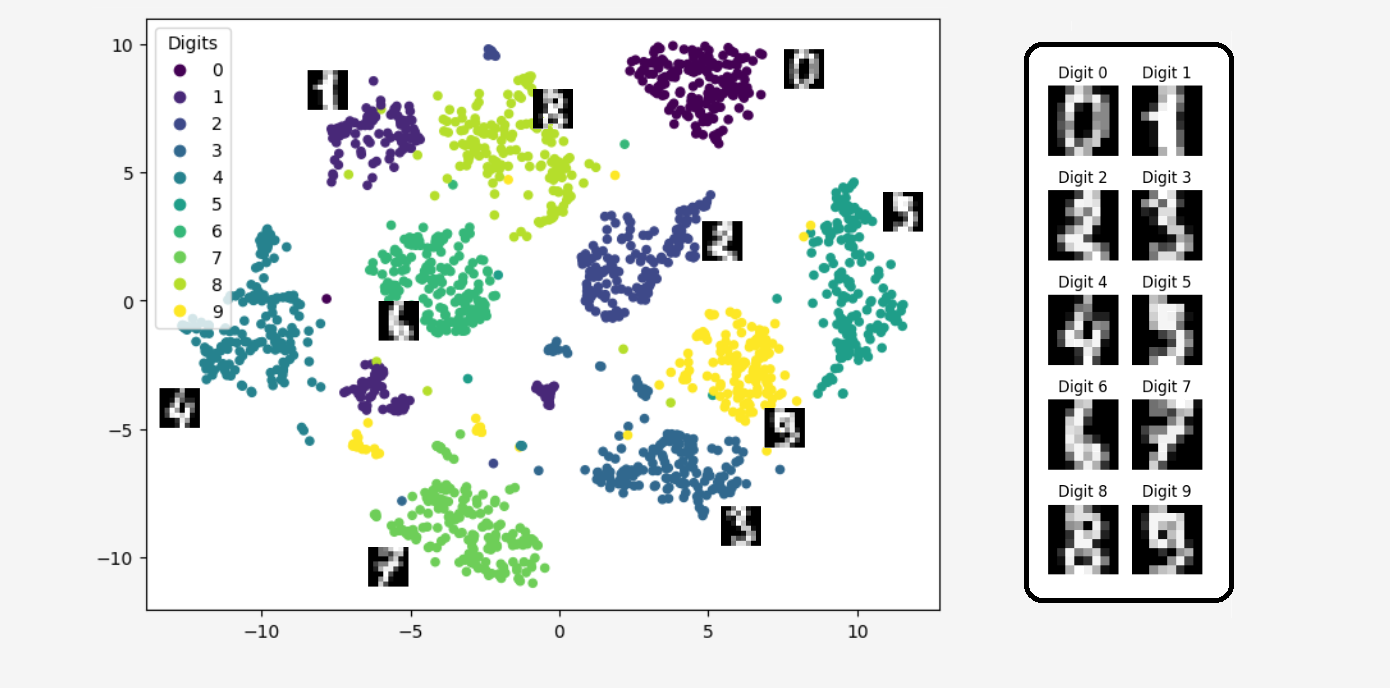
Let's take a well-known dataset in the machine learning community, containing nearly 1800 images with a resolution of \(8 \times 8\), representing handwritten digits from 0 to 9. An \(8 \times 8\) resolution means that the two-dimensional image consists of \(64 = 8\cdot 8\) pixels, each in grayscale, with a value ranging from 0 (black) to 255 (white). Therefore, each image is described by 64 variables. We can say that each observation comes from a 64-dimensional space.
Let's see what we get when we use the t-SNE algorithm to reduce the dimensionality from 64 to just 2 dimensions!

from sklearn.datasets import load_digits
import matplotlib.pyplot as plt
X, y = load_digits(return_X_y=True)

res = tsne(X,  ydim=2, iterations=100, learning_rate=500, perplexity=30)

plt.figure(figsize=(8, 6))
scatter = plt.scatter(res[:, 0], res[:, 1], s=20, c=y)
plt.legend(
  handles=scatter.legend_elements()[0],
  labels=[str(i) for i in np.unique(y)],
  title="Digits"
  )
plt.show()

Isn't it amazing?
The algorithm transformed 64-dimensional data into two dimensions in such a way that we can still distinguish between the different digits. Thus, the data transformed using the t-SNE algorithm didn’t lose much information; in fact, the information from the 64 dimensions was compressed into just two dimensions!

Advantages and Disadvantages of t-SNE

Let's summarize once again why t-SNE is such a great algorithm.

Advantages

1. Visualization
   t-SNE is brilliant at visualizing data in 2D space, which allows for a better understanding of clusters and groups in the data.
2. Local Structures
   t-SNE maintains similarities between data points in higher dimensions, attempting to map local neighborhoods into 2D space.
3. High flexibility
   It can be applied in various fields, such as image analysis, text analysis to visualize complex datasets.

However, to temper your enthusiasm a bit, we must also mention the drawbacks of the algorithm.

Disadvantages

1. Lack of a clear method for evaluating result quality
   t-SNE can be very slow with large datasets because it computes distances between all pairs of points
2. Problems with clusters of very different densities
   Unlike some other algorithms, t-SNE does not have a definitive criterion for assessing the quality of the mapping to lower-dimensional space, making it difficult to evaluate the model's effectiveness.
3. Sensitivity to hyperparameters
   The choice of appropriate parameters can significantly affect the quality of the results. This often requires a lot of experimentation to achieve optimal visualization.

Conclusion:

t-SNE (t-Distributed Stochastic Neighbor Embedding) is a powerful technique for visualizing high-dimensional data by reducing it to two or three dimensions. It builds on the earlier Stochastic Neighbor Embedding algorithm, addressing its limitations and improving its ability to represent relationships in low-dimensional spaces.

From SNE to t-SNE:
SNE minimizes the Kullback-Leibler divergence between the conditional probabilities of pairwise similarities in high- and low-dimensional spaces. While effective, it suffers from challenges such as the "crowding problem," where moderately distant points are compressed too closely in the low-dimensional representation.

Key Improvements in t-SNE:
• SNE used asymmetric probabilities, which introduced inconsistencies in how relationships were represented. Symmetric SNE (s-SNE) resolved this by making the similarity measure symmetric, improving optimization stability.
• To mitigate the crowding problem, t-SNE replaces the Gaussian kernel used in SNE's low-dimensional space with a t-distribution. The heavy tails of the t-distribution allow for better representation of moderately distant points by creating stronger repulsive forces between them.

Interpretation of Results:
• t-SNE focuses on preserving local neighborhoods rather than absolute distances. Points that are close in the high-dimensional space remain close in the low-dimensional embedding.
• The algorithm sacrifices global structure for local fidelity, making it well-suited for visualizing clusters and relationships but less reliable for interpreting large-scale distances.

Practical Considerations:
• The choice of perplexity, a parameter controlling the balance between local and global relationships, significantly affects the results.
• Computational complexity grows with the number of data points, though modern implementations like Barnes-Hut t-SNE alleviate this issue.


See You! 😁

References

• G. Hinton, S. Roweis, Stochastic Neighbor Embedding
• L.J.P. van der Maaten, G. Hinton, Visualizing Data using t-SNE