From Theory to Practice:
Ridge Regression for Improved Predictive Models

---

Ridge regression is a modification of linear regression, so a good understanding of linear regression will certainly help you better understand the article below.

Ridge Regression - short introduction

Ridge regression is a variation of linear regression, specifically designed to address multicollinearity in the dataset. In linear regression, as we know, the goal is to find the best-fitting hyperplane that minimizes the sum of squared differences between the observed and predicted values. However, when there are highly correlated variables, linear regression may become unstable and provide unreliable estimates.

Multicollinearity exists when two or more of the predictors in a regression model are moderately or highly correlated with one another.

Ridge regression introduces a regularization term that penalizes large coefficients, helping to stabilize the model and prevent overfitting. This regularization term, also known as the L2 penalty, adds a constraint to the optimization process, influencing the model to choose smaller coefficients for the predictors. By striking a balance between fitting the data well and keeping the coefficients in check, ridge regression proves valuable in improving the robustness and performance of linear regression models, especially in situations with multicollinearity.

We will explain all these peculiar terms in a moment 😁

Linear Regression - What It's All About?

Let's briefly recall what linear regression was about.

In linear regression, the model training essentially involves finding the appropriate values for coefficients. This is done using the method of least squares. One seeks the values \(\beta_0, \beta_1,...,\beta_p\) that minimize the Residual Sum of Squares: $$RSS=\sum_{i=1}^{n}\left( y_i-\beta_0-\sum_{j=1}^{p}\beta_jx_{ij} \right)^2$$ Using matrix notation and taking advantage of the benefits of differential calculus, we sought an explicit formula for the coefficients \(\beta_j\).

Ridge Regression - definition

Ridge regression is very similar to the method of least squares, with the exception that the coefficients are estimated by minimizing a slightly different quantity. In reality, it's the same quantity, just with something more, with something we call a shrinkage penalty. $$\sum_{i=1}^{n}\left( y_i-\beta_0-\sum_{j=1}^{p}\beta_jx_{ij} \right)^2+\lambda\sum_{j=1}^{p}\beta_{j}^2=RSS+\lambda\sum_{j=1}^{p}\beta_{j}^2$$ Before we explain what ridge regression is, let's find out what the mysterious shrinkage penalty is all about.

Shrinkage penalty - aid in learning

The shrinkage penalty in ridge regression $$\lambda\sum_{j=1}^{p}\beta_{j}^2$$ refers to the regularization term added to the linear regression equation to prevent overfitting and address multicollinearity. In ridge regression, the objective is to minimize the sum of squared differences between observed and predicted values. However, to this, a penalty term is added, which is proportional to the square of the magnitude of the coefficients. This penalty term is also known as the \(\ell_2\) norm or Euclidean norm.

Parameter \(\lambda \ge 0\) is called the tuning parameter of the method, which is chosen separately. The parameter \(\lambda\) controls how strongly the coefficients are shrunk toward 0. When \(\lambda = 0\), the penalty has no effect, and ridge regression reduces to the ordinary least squares method - just linear regression. However, as \(\lambda \to \infty\) the impact of the penalty grows, and the estimates of the coefficients \(\beta_j\) in ridge regression shrink towards zero.

How to choose \(\lambda\)?

How to determine which value of \(\lambda\) to use?
You might not like the answer. At the beginning, it's not known. The only way is to test many values, and that's typically how it's done. However, there are many algorithm implementations that assist in selecting the appropriate \(\lambda\) like cross-validation.

A standard approach is to define a grid of candidate values, for example a sequence that is evenly spaced on the \(\log(\lambda)\) scale. For each value on this grid, the ridge model is fit and its performance is evaluated, typically using mean squared error.
The most common strategy is cross-validation. We have already become familiar with this method - it was described in the previous article.. The data are split into \(K\) approximately equal parts. In each round, one part is used as a validation set while the model is trained on the remaining \(K-1\) parts, and this procedure is repeated for all folds and all candidate values of \(\lambda\).
Let's look at an example plot of MSE errors versus \(\log(\lambda)\):
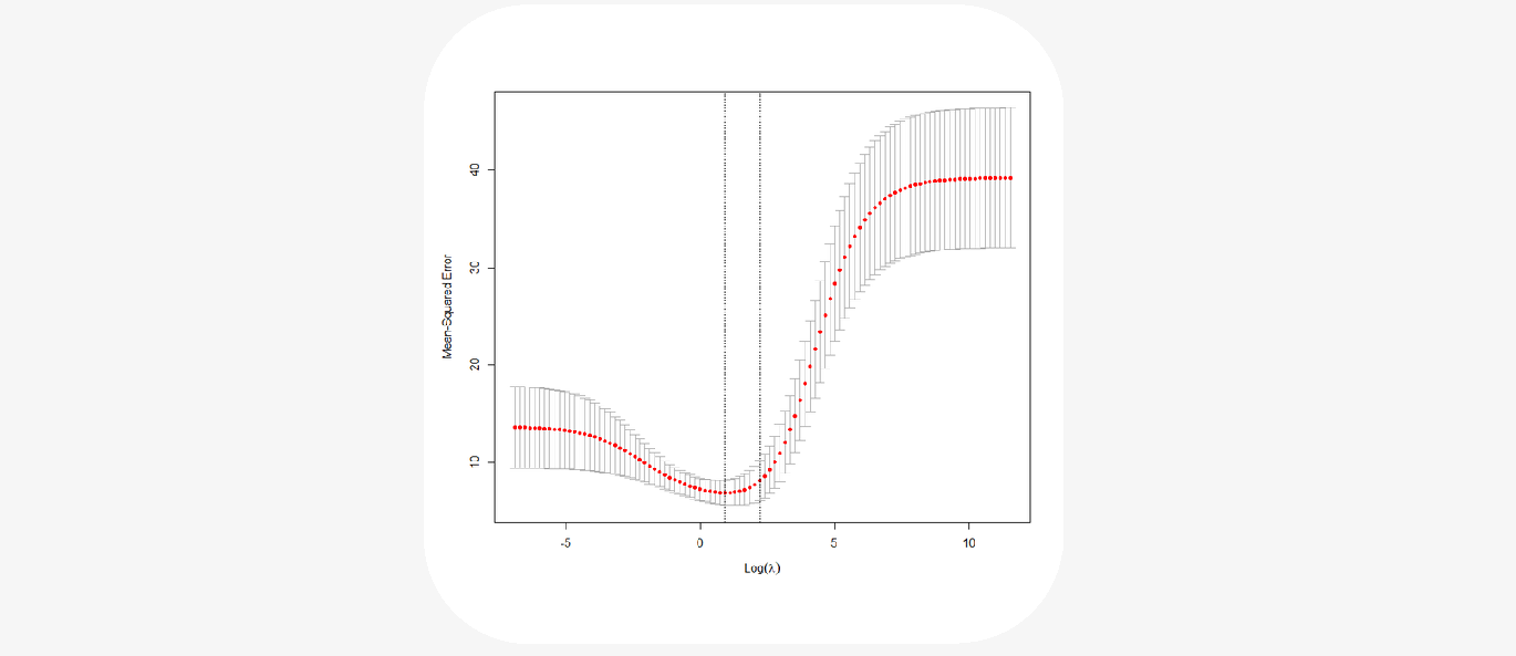
In practice, \(\lambda\) is chosen near the minimum of the validation curve (sometimes using the one-standard-deviation rule), and then the ridge model is refit on the entire training set using this selected parameter value.

Why you should scale predictors?

It should also be noted that the shrinkage penalty is applied exclusively to the coefficients \(\beta_1, ..., \beta_p\), but it does not affect the intercept term \(\beta_0\). We do not shrink the intercept - it represents the prediction of the mean value of the dependent variable when all predictors are equal to 0. Assuming that the variables have been centered to have a mean of zero before conducting ridge regression, the estimated intercept will take the form $$\beta_0=\frac{1}{n}\sum_{i=1}^{n}y_i$$ It should be emphasized that scaling predictors matters. In linear regression, multiplying the predictor \(X_j\) by a constant \(c\) reduces the estimated parameter by \(1/c\) (meaning \(X_j\beta_j\) remains unchanged). However, in ridge regression, due to the shrinkage penalty, scaling the predictor \(X_j\) can significantly change both the estimated parameter \(\beta_j\) and other predictors. Therefore, before applying ridge regression, predictors are standardized to be on the same scale.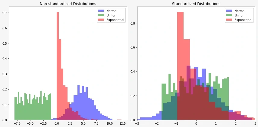

Feature standardization is a preprocessing step in machine learning where the input features are transformed to have a mean of 0 and a standard deviation of 1. This is typically achieved by subtracting the mean of each feature from its values and then dividing by the standard deviation.

If the population mean and population standard deviation are known, a raw variable \(x\) is converted into a standard score by $$z=\frac{x-\mu}{\sigma}$$ Let's try to understand this with an example:
If one of the variables is the price of an apartment (in hundreds of thousands) and the other is the number of rooms in that apartment (in units), it's difficult to compare both quantities. After standardization, their variables will have similar values (though somewhat abstract), but their distribution won't change.

The primary reasons for feature standardization are:
• Magnitude Consistency:
Machine learning models that rely on distances or gradients, such as gradient descent-based optimization algorithms, are sensitive to the scale of the input features. Standardizing features ensures that all features contribute equally to the model, preventing some features from dominating others based solely on their scale.

• Convergence Speed:
Standardizing features can lead to faster convergence during the training of models. Optimization algorithms often converge more quickly when the features are on a similar scale, as it helps the algorithm navigate the parameter space more efficiently.

• Numerical Stability:
Standardization can enhance the numerical stability of computations. Large-scale differences in the ranges of features may lead to numerical precision issues, especially in models that involve matrix operations or exponentiation.

• Regularization Effectiveness:
In models that involve regularization, such as ridge regression or lasso regression, feature standardization ensures that the regularization term applies uniformly to all features. This helps prevent the model from assigning disproportionately large weights to certain features.

While feature standardization is beneficial in many cases, it may not be necessary for all machine learning algorithms. For instance, decision tree-based models are generally insensitive to the scale of features. However, for algorithms like support vector machines, k-nearest neighbors, and linear models feature standardization is often recommended.

How to estimate coefficients in ridge regression?

Just as in the case of regression, where we minimized the RSS, for ridge regression, we minimize the expression we mentioned earlier, but this time let's express it in matrix form: $$RSS_\operatorname{Ridge}=(\mathbf{Y}-\mathbf{X}\beta)^T(\mathbf{Y}-\mathbf{X}\beta)+\lambda\beta^T\beta=||\mathbf{Y}-\mathbf{X}\beta||^2+\lambda||\beta||^2$$ To minimize the \(RSS_\operatorname{Ridge}\) expression, we will set its derivative (with respect to \(\beta\)) equal to zero. $$\nabla RSS_\operatorname{Ridge}=-2\mathbf{X}^T(\mathbf{Y}-\mathbf{X}\beta)+2\lambda\mathbf{I}\beta=0$$ Hence $$-2\left( \mathbf{X}^T(\mathbf{Y}-\mathbf{X}\beta)-\lambda\mathbf{I}\beta \right)=0$$ $$\mathbf{X}^T(\mathbf{Y}-\mathbf{X}\beta)-\lambda\mathbf{I}\beta=0$$ $$\mathbf{X}^T\mathbf{Y}-\mathbf{X}^T\mathbf{X}\beta+\lambda\mathbf{I}\beta=0$$ $$(\mathbf{X}^T\mathbf{X}+\lambda\mathbf{I})\beta=\mathbf{X}^T\mathbf{Y}$$ The matrix \(\mathbf{X}^T\mathbf{X}+\lambda\mathbf{I}\) has full rank and it is invertible. As a consequence: $$\beta=(\mathbf{X}^T\mathbf{X}+\lambda\mathbf{I})^{-1}\mathbf{X}^T\mathbf{Y}$$ Now we need to check that this is indeed a global minimum. Note that the Hessian matrix, the matrix of second derivatives of \(RSS_\operatorname{Ridge}\), is positive definite. $$\nabla^2 RSS_\operatorname{Ridge}=2\mathbf{X}^T\mathbf{X}+2\lambda\mathbf{I}$$ Then, \(RSS_\operatorname{Ridge}\) is strictly convex, which implies that this is a global minimum.

Bias–variance tradeoff of the ridge estimator

The superiority of ridge regression compared to the method of least squares arises from the inherent trade-off between variance and bias. Ridge regression introduces a regularization parameter, denoted as \(\lambda\), which controls the extent of shrinkage applied to the regression coefficients. As the value of \(\lambda\) increases, the model's flexibility in fitting the data diminishes. Consequently, this decrease in flexibility results in a simultaneous reduction in variance but an increase in bias.

In other words, ridge regression provides a means to strike a balance between the precision of fitting the training data and the generalizability of the model to new, unseen data. By introducing a penalty term associated with the size of the coefficients, ridge regression prevents the model from becoming overly complex and sensitive to noise in the training data. This regularization mechanism becomes particularly valuable in scenarios where multicollinearity is present, contributing to a stabilized and more reliable model.

• When the number of predictors, \(p\), is close to the number of observations, \(n\), the method of least squares exhibits high variance – a small change in the training data can lead to a significant change in the estimated parameters.
• When \(p > n\), the method of least squares stops working (due to the lack of estimation uniqueness), whereas ridge regression handles this situation exceptionally well.

It's time for an example.

Example

Here, the genetic markers represent variations at specific genomic locations, and the trait is a quantitative measure associated with a particular individual.

Suppose we have a dataset with genetic markers (A, B, C, D, E) as predictors and a trait (T) as the response variable.

The dataset looks like this:

Marker A	Marker B	Marker C	Marker D	Marker E	Trait
0.8	1.2	0.5	-0.7	1.0	3.2
1.0	0.8	-0.4	0.5	-1.2	2.5
-0.5	0.3	1.2	0.9	-0.1	1.8
0.2	-0.9	-0.7	1.1	0.5	2.9

At the beginning, we need to specify the value of the hyperparameter for our method, which is \(\lambda\).
Let \(\lambda=2\).

Taking data from the example, the matrix \(\mathbf{X}_{\operatorname{RAW}}\) takes the form: $$ \mathbf{X}_{\operatorname{RAW}} = \left( \begin{array}{ccccc} 0.8 & 1.2 & 0.5 & -0.7 & 1.0 \\ 1.0 & 0.8 & -0.4 & 0.5 & -1.2 \\ -0.5 & 0.3 & 1.2 & 0.9 & -0.1 \\ 0.2 & -0.9 & -0.7 & 1.1 & 0.5 \\ \end{array} \right) $$ We remember that before creating a ridge regression model, we need to standardize the predictors so that they all have a mean of zero and a standard deviation of 1. Using a simple formula for the \(z\)-score: $$z=\frac{x-\mu}{\sigma}$$ We obtain a matrix of data after standardizing the predictors. $$ \mathbf{X} = \left( \begin{array}{ccccc} 0.72686751 & 1.07733123 & 0.46666667 & -1.64706421 & 1.15845045 \\ 1.06892281 & 0.57035183 & -0.73333333 & 0.07161149 & -1.5242769 \\ -1.49649194 & -0.06337243 & 1.4 & 0.64450339 & -0.18291323 \\ -0.29929839 & -1.58431063 & -1.13333333 & 0.93094934 & 0.54873968 \\ \end{array} \right) $$ Unfortunately, after standardization, the numbers may not be convenient for calculations. Usually, the computer handles the computations for us, but if we want to trace step by step how ridge regression works, we have to deal with inconvenient numbers.

To build a ridge regression model essentially means to find the coefficients \(\beta\) (as \(\beta\) we understand the vector of coefficients \((\beta_1,...\beta_p\))). From our previous considerations, we already know the recipe to obtain them: $$\beta=(\mathbf{X}^T\mathbf{X}+\lambda\mathbf{I})^{-1}\mathbf{X}^T\mathbf{Y}$$ So, first, we need to multiply the transposed matrix \(X^T\) by the matrix \(X\), and then add to it the scaled identity matrix \(\mathbf{I}\), scaled by the hyperparameter \(\lambda\) (in our case \(\lambda=2\)). $$ \mathbf{X}^T\mathbf{X}+\lambda\mathbf{I} = \left( \begin{array}{ccccc} 6. & 1.96175708 & -2.20055576 & -2.36377607 & -0.67780309 \\ 1.96175708 & 6. & 1.79132721 & -3.24934663 & -0.47912173 \\ -2.20055576 & 1.79132721 & 6. & -0.97391623 & 0.78042977 \\ -2.36377607 & -3.24934663 & -0.97391623 & 6. & -1.62423735 \\ -0.67780309 & -0.47912173 & 0.78042977 & -1.62423735 & 6. \\ \end{array} \right) $$ Then we need to invert it. $$ (\mathbf{X}^T\mathbf{X}+\lambda\mathbf{I})^{-1} = \left( \begin{array}{ccccc} 0.28919553 & -0.07688096 & 0.14132356 & 0.10514749 & 0.03661227 \\ -0.07688096 & 0.30018168 & -0.1046914 & 0.13284326 & 0.06486445 \\ 0.14132356 & -0.1046914 & 0.25776258 & 0.03647517 & -0.01604861 \\ 0.10514749 & 0.13284326 & 0.03647517 & 0.3137487 & 0.10267557 \\ 0.03661227 & 0.06486445 & -0.01604861 & 0.10267557 & 0.2058647 \\ \end{array} \right) $$ And finally, multiply, first by \(X^T\), and then by \(Y\). 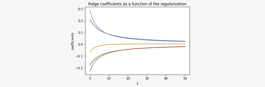We will then obtain: $$ \beta = \left( \begin{array}{c} 0.1593035 \\ -0.03361389 \\ -0.16299572 \\ -0.13492445 \\ 0.19306318 \\ \end{array} \right) $$ Notice that the results depend on the value of \(\lambda\). If we change \(\lambda\), we will get a different result. In the plot below, we can observe how the estimated values of coefficients \(\beta\) change depending on the chosen parameter \(\lambda\).


We estimated coefficients \(\beta_1, ..., \beta_p\), but what about the intercept term \(\beta_0\)? We mentioned that assuming the variables have been centered to have a mean of zero before conducting ridge regression, the estimated intercept will take the form: $$\beta_0=\frac{1}{n}\sum_{i=1}^{n}y_i$$ In our case $$\beta_0=\frac{3.2+2.5+1.8+2.9}{4}=2.6$$ Now, to calculate predictions, we need to apply the formula: $$\mathbf{\hat{Y}} = \mathbf{X} \beta +\beta_0$$ If we wanted to predict the values of the target variable using our model, we would obtain the following values: $$ \mathbf{\hat{Y}} = \mathbf{X} \beta +\beta_0=$$ $$=\left( \begin{array}{ccccc} 0.72686751 & 1.07733123 & 0.46666667 & -1.64706421 & 1.15845045 \\ 1.06892281 & 0.57035183 & -0.73333333 & 0.07161149 & -1.5242769 \\ -1.49649194 & -0.06337243 & 1.4 & 0.64450339 & -0.18291323 \\ -0.29929839 & -1.58431063 & -1.13333333 & 0.93094934 & 0.54873968 \\ \end{array} \right) \left( \begin{array}{c} 0.1593035 \\ -0.03361389 \\ -0.16299572 \\ -0.13492445 \\ 0.19306318 \\ \end{array} \right) + \left( \begin{array}{c} 2.6 \\ 2.6 \\ 2.6 \\ 2.6 \\ 2.6 \\ \end{array} \right) =$$ $$= \left( \begin{array}{c} 3.04939794 \\ 2.56669771 \\ 2.01326671 \\ 2.77063765 \end{array} \right) $$ We can now compare our predictions with the actual values to demonstrate that the calculations lead to good results. $$ \mathbf{\hat{Y}}= \left( \begin{array}{c} 3.04939794 \\ 2.56669771 \\ 2.01326671 \\ 2.77063765 \end{array} \right) \hspace{10mm} \mathbf{Y}= \left( \begin{array}{c} 3.2 \\ 2.5 \\ 1.8 \\ 2.9 \end{array} \right) $$

Implementation - Ridge Regression

Now, we will focus on implementing our ridge regression. We will do it step by step using the Python language. We won't use classes to avoid obscuring what's most important, which is a thorough understanding of how the algorithm works. Thanks to this, beginners will be able to execute the code line by line and understand it.

To start, let's generate a dataset, exactly the same as in the example from the previous chapter. Before that, let's also import the necessary libraries.
We also need to remember to define the hyperparameter of our algorithm, which is the shrinkage parameter \(\lambda\). Just like in the example, let's assume \(\lambda=2\).

import numpy as np

LAMBDA = 2

X = np.array([[0.8,  1.2,  0.5,  -0.7, 1.0],
              [1.0,  0.8,  -0.4, 0.5,  -1.2],
              [-0.5, 0.3,  1.2,  0.9,  -0.1],
              [0.2,  -0.9, -0.7, 1.1,  0.5]])

y = np.array([3.2, 2.5, 1.8, 2.9])

Of course, we must remember that before creating a ridge regression model, we need to standardize the predictors so that they all have a mean of zero and a standard deviation of 1. We will use the formula for the z-score: $$z=\frac{x-\mu}{\sigma}$$

X_scale = (X-X.mean(axis=0))/X.std(axis=0)

To build a ridge regression model essentially means to find the coefficients. From the theoretical part, we learned how we can obtain these coefficients. It is enough to use the formula: $$\beta=(\mathbf{X}^T\mathbf{X}+\lambda\mathbf{I})^{-1}\mathbf{X}^T\mathbf{Y}$$ For clarity, we will break down this section into smaller steps so that each operation on matrices can be traced.
The function \(\texttt{inv()}\) comes from the \(\texttt{numpy.linalg}\) module. It calculates the inverse of a matrix. Meanwhile, the function \(\texttt{np.identity(5)}\) creates an identity matrix of size \(5\times5\) (because we have 5 variables).

# X*X^T + LAMBDA*I
x1 = np.matmul(X_scale.T, X_scale) + LAMBDA*np.identity(5)
# Transpose obtained matrix - (X*X^T + LAMBDA*I)^{-1}
x1_inv = np.linalg.inv(x1)
# ( (X*X^T + LAMBDA*I)^{-1} ) * X^T
x2 = np.matmul(x1_inv, X_scale.T)
# ( ( (X*X^T + LAMBDA*I)^{-1} ) * X^T ) * Y
coef = np.matmul(x2, y)
# Estimated coeficients
print(coef)

We obtained the following coefficients, exactly the same as in the example from the previous section.

[0.1593035  -0.03361389 -0.16299572 -0.13492445  0.19306318]

To calculate predictions, we need to apply the formula \(\mathbf{\hat{Y}} = \mathbf{X} \beta +\beta_0\)
From previous considerations we remember that \(\beta_0\) is simply the mean value of the target variable.

np.matmul(X_scale, coef)+y.mean()

Finally, here's the entire code again:

import numpy as np

LAMBDA = 2    # shrinkage parameter

# Define dataset (X,y)
X = np.array([[0.8,  1.2,  0.5,  -0.7, 1.0],
              [1.0,  0.8,  -0.4, 0.5,  -1.2],
              [-0.5, 0.3,  1.2,  0.9,  -0.1],
              [0.2,  -0.9, -0.7, 1.1,  0.5]])

y = np.array([3.2, 2.5, 1.8, 2.9])

# Scale predictors
X_scale = (X-X.mean(axis=0))/X.std(axis=0)

# RIDGE REGRESSION MODEL - coefficients estimation
# X*X^T + LAMBDA*I
x1 = np.matmul(X_scale.T, X_scale) + LAMBDA*np.identity(5)
# Transpose obtained matrix - (X*X^T + LAMBDA*I)^{-1}
x1_inv = np.linalg.inv(x1)
# ( (X*X^T + LAMBDA*I)^{-1} ) * X^T
x2 = np.matmul(x1_inv, X_scale.T)
# ( ( (X*X^T + LAMBDA*I)^{-1} ) * X^T ) * Y
coef = np.matmul(x2, y)
# Estimated coeficients
print(coef)

# predictions
np.matmul(X_scale, coef)+y.mean()

Conclusion:

In this blog post, we explored the concept of ridge regression, a valuable technique in regression analysis, particularly useful when dealing with multicollinearity or situations where the number of predictors exceeds the number of observations. By introducing a regularization term controlled by the hyperparameter \(\lambda\), ridge regression strikes a balance between variance and bias, leading to more stable and reliable models.

We discussed the key steps involved in ridge regression, from standardizing predictors to estimating coefficients and making predictions. Through simple examples and explanations, we demonstrated how ridge regression works, emphasizing its ability to handle challenging scenarios such as high-dimensional data or correlated predictors.

Furthermore, we highlighted the importance of selecting an appropriate value for the hyperparameter \(\lambda\) and showcased how different values of \(\lambda\) influence the estimated coefficients and, consequently, the model's predictions.

Overall, ridge regression offers a powerful tool for improving the robustness and performance of linear regression models, making it a valuable technique in the toolkit of data scientists and analysts working with regression problems. By understanding its principles and applications, practitioners can leverage ridge regression to build more accurate and reliable predictive models in various domains.

Happy learning! 😁